Probability distribution
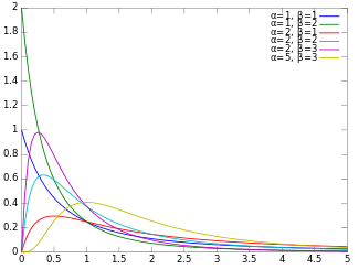
Probability density function
Cumulative distribution function
Parameters
α
>
0
{\displaystyle \alpha >0}
shape (real )
β
>
0
{\displaystyle \beta >0}
Support
x
∈
[
0
,
∞
)
{\displaystyle x\in [0,\infty )\!}
PDF
f
(
x
)
=
x
α
−
1
(
1
+
x
)
−
α
−
β
B
(
α
,
β
)
{\displaystyle f(x)={\frac {x^{\alpha -1}(1+x)^{-\alpha -\beta }}{B(\alpha ,\beta )}}\!}
CDF
I
x
1
+
x
(
α
,
β
)
{\displaystyle I_{{\frac {x}{1+x}}(\alpha ,\beta )}}
I
x
(
α
,
β
)
{\displaystyle I_{x}(\alpha ,\beta )}
Mean
α
β
−
1
if
β
>
1
{\displaystyle {\frac {\alpha }{\beta -1}}{\text{ if }}\beta >1}
Mode
α
−
1
β
+
1
if
α
≥
1
, 0 otherwise
{\displaystyle {\frac {\alpha -1}{\beta +1}}{\text{ if }}\alpha \geq 1{\text{, 0 otherwise}}\!}
Variance
α
(
α
+
β
−
1
)
(
β
−
2
)
(
β
−
1
)
2
if
β
>
2
{\displaystyle {\frac {\alpha (\alpha +\beta -1)}{(\beta -2)(\beta -1)^{2}}}{\text{ if }}\beta >2}
Skewness
2
(
2
α
+
β
−
1
)
β
−
3
β
−
2
α
(
α
+
β
−
1
)
if
β
>
3
{\displaystyle {\frac {2(2\alpha +\beta -1)}{\beta -3}}{\sqrt {\frac {\beta -2}{\alpha (\alpha +\beta -1)}}}{\text{ if }}\beta >3}
MGF
Does not exist CF
e
−
i
t
Γ
(
α
+
β
)
Γ
(
β
)
G
1
,
2
2
,
0
(
α
+
β
β
,
0
|
−
i
t
)
{\displaystyle {\frac {e^{-it}\Gamma (\alpha +\beta )}{\Gamma (\beta )}}G_{1,2}^{\,2,0}\!\left(\left.{\begin{matrix}\alpha +\beta \\\beta ,0\end{matrix}}\;\right|\,-it\right)}
In probability theory and statistics , the beta prime distribution (also known as inverted beta distribution or beta distribution of the second kind [1] absolutely continuous probability distribution . If
p
∈
[
0
,
1
]
{\displaystyle p\in [0,1]}
beta distribution , then the odds
p
1
−
p
{\displaystyle {\frac {p}{1-p}}}
Definitions Beta prime distribution is defined for
x
>
0
{\displaystyle x>0}
α and β , having the probability density function :
f
(
x
)
=
x
α
−
1
(
1
+
x
)
−
α
−
β
B
(
α
,
β
)
{\displaystyle f(x)={\frac {x^{\alpha -1}(1+x)^{-\alpha -\beta }}{B(\alpha ,\beta )}}}
where B is the Beta function .
The cumulative distribution function is
F
(
x
;
α
,
β
)
=
I
x
1
+
x
(
α
,
β
)
,
{\displaystyle F(x;\alpha ,\beta )=I_{\frac {x}{1+x}}\left(\alpha ,\beta \right),}
where I is the regularized incomplete beta function .
The expected value, variance, and other details of the distribution are given in the sidebox; for
β
>
4
{\displaystyle \beta >4}
excess kurtosis is
γ
2
=
6
α
(
α
+
β
−
1
)
(
5
β
−
11
)
+
(
β
−
1
)
2
(
β
−
2
)
α
(
α
+
β
−
1
)
(
β
−
3
)
(
β
−
4
)
.
{\displaystyle \gamma _{2}=6{\frac {\alpha (\alpha +\beta -1)(5\beta -11)+(\beta -1)^{2}(\beta -2)}{\alpha (\alpha +\beta -1)(\beta -3)(\beta -4)}}.}
While the related beta distribution is the conjugate prior distribution of the parameter of a Bernoulli distribution expressed as a probability, the beta prime distribution is the conjugate prior distribution of the parameter of a Bernoulli distribution expressed in odds . The distribution is a Pearson type VI distribution.[1]
The mode of a variate X distributed as
β
′
(
α
,
β
)
{\displaystyle \beta '(\alpha ,\beta )}
X
^
=
α
−
1
β
+
1
{\displaystyle {\hat {X}}={\frac {\alpha -1}{\beta +1}}}
α
β
−
1
{\displaystyle {\frac {\alpha }{\beta -1}}}
β
>
1
{\displaystyle \beta >1}
β
≤
1
{\displaystyle \beta \leq 1}
α
(
α
+
β
−
1
)
(
β
−
2
)
(
β
−
1
)
2
{\displaystyle {\frac {\alpha (\alpha +\beta -1)}{(\beta -2)(\beta -1)^{2}}}}
β
>
2
{\displaystyle \beta >2}
For
−
α
<
k
<
β
{\displaystyle -\alpha <k<\beta }
k -th moment
E
[
X
k
]
{\displaystyle E[X^{k}]}
E
[
X
k
]
=
B
(
α
+
k
,
β
−
k
)
B
(
α
,
β
)
.
{\displaystyle E[X^{k}]={\frac {B(\alpha +k,\beta -k)}{B(\alpha ,\beta )}}.}
For
k
∈
N
{\displaystyle k\in \mathbb {N} }
k
<
β
,
{\displaystyle k<\beta ,}
E
[
X
k
]
=
∏
i
=
1
k
α
+
i
−
1
β
−
i
.
{\displaystyle E[X^{k}]=\prod _{i=1}^{k}{\frac {\alpha +i-1}{\beta -i}}.}
The cdf can also be written as
x
α
⋅
2
F
1
(
α
,
α
+
β
,
α
+
1
,
−
x
)
α
⋅
B
(
α
,
β
)
{\displaystyle {\frac {x^{\alpha }\cdot {}_{2}F_{1}(\alpha ,\alpha +\beta ,\alpha +1,-x)}{\alpha \cdot B(\alpha ,\beta )}}}
where
2
F
1
{\displaystyle {}_{2}F_{1}}
hypergeometric function 2 F1 .
Alternative parameterization The beta prime distribution may also be reparameterized in terms of its mean μ > 0 and precision ν > 0 parameters ([2]
Consider the parameterization μ = α /(β -1) and ν = β - 2, i.e., α = μ ( 1 + ν ) and
β = 2 + ν . Under this parameterization
E[Y] = μ and Var[Y] = μ (1 + μ )/ν .
Generalization Two more parameters can be added to form the generalized beta prime distribution
β
′
(
α
,
β
,
p
,
q
)
{\displaystyle \beta '(\alpha ,\beta ,p,q)}
p
>
0
{\displaystyle p>0}
shape (real )
q
>
0
{\displaystyle q>0}
real )having the probability density function :
f
(
x
;
α
,
β
,
p
,
q
)
=
p
(
x
q
)
α
p
−
1
(
1
+
(
x
q
)
p
)
−
α
−
β
q
B
(
α
,
β
)
{\displaystyle f(x;\alpha ,\beta ,p,q)={\frac {p\left({\frac {x}{q}}\right)^{\alpha p-1}\left(1+\left({\frac {x}{q}}\right)^{p}\right)^{-\alpha -\beta }}{qB(\alpha ,\beta )}}}
with mean
q
Γ
(
α
+
1
p
)
Γ
(
β
−
1
p
)
Γ
(
α
)
Γ
(
β
)
if
β
p
>
1
{\displaystyle {\frac {q\Gamma \left(\alpha +{\tfrac {1}{p}}\right)\Gamma (\beta -{\tfrac {1}{p}})}{\Gamma (\alpha )\Gamma (\beta )}}\quad {\text{if }}\beta p>1}
and mode
q
(
α
p
−
1
β
p
+
1
)
1
p
if
α
p
≥
1
{\displaystyle q\left({\frac {\alpha p-1}{\beta p+1}}\right)^{\tfrac {1}{p}}\quad {\text{if }}\alpha p\geq 1}
Note that if p = q = 1 then the generalized beta prime distribution reduces to the standard beta prime distribution .
This generalization can be obtained via the following invertible transformation. If
y
∼
β
′
(
α
,
β
)
{\displaystyle y\sim \beta '(\alpha ,\beta )}
x
=
q
y
1
/
p
{\displaystyle x=qy^{1/p}}
q
,
p
>
0
{\displaystyle q,p>0}
x
∼
β
′
(
α
,
β
,
p
,
q
)
{\displaystyle x\sim \beta '(\alpha ,\beta ,p,q)}
Compound gamma distribution The compound gamma distribution [3] q is added, but where p = 1. It is so named because it is formed by compounding two gamma distributions :
β
′
(
x
;
α
,
β
,
1
,
q
)
=
∫
0
∞
G
(
x
;
α
,
r
)
G
(
r
;
β
,
q
)
d
r
{\displaystyle \beta '(x;\alpha ,\beta ,1,q)=\int _{0}^{\infty }G(x;\alpha ,r)G(r;\beta ,q)\;dr}
where
G
(
x
;
a
,
b
)
{\displaystyle G(x;a,b)}
a
{\displaystyle a}
b
{\displaystyle b}
The mode, mean and variance of the compound gamma can be obtained by multiplying the mode and mean in the above infobox by q and the variance by q 2 .
Another way to express the compounding is if
r
∼
G
(
β
,
q
)
{\displaystyle r\sim G(\beta ,q)}
x
∣
r
∼
G
(
α
,
r
)
{\displaystyle x\mid r\sim G(\alpha ,r)}
x
∼
β
′
(
α
,
β
,
1
,
q
)
{\displaystyle x\sim \beta '(\alpha ,\beta ,1,q)}
Properties If
X
∼
β
′
(
α
,
β
)
{\displaystyle X\sim \beta '(\alpha ,\beta )}
1
X
∼
β
′
(
β
,
α
)
{\displaystyle {\tfrac {1}{X}}\sim \beta '(\beta ,\alpha )}
If
Y
∼
β
′
(
α
,
β
)
{\displaystyle Y\sim \beta '(\alpha ,\beta )}
X
=
q
Y
1
/
p
{\displaystyle X=qY^{1/p}}
X
∼
β
′
(
α
,
β
,
p
,
q
)
{\displaystyle X\sim \beta '(\alpha ,\beta ,p,q)}
If
X
∼
β
′
(
α
,
β
,
p
,
q
)
{\displaystyle X\sim \beta '(\alpha ,\beta ,p,q)}
k
X
∼
β
′
(
α
,
β
,
p
,
k
q
)
{\displaystyle kX\sim \beta '(\alpha ,\beta ,p,kq)}
β
′
(
α
,
β
,
1
,
1
)
=
β
′
(
α
,
β
)
{\displaystyle \beta '(\alpha ,\beta ,1,1)=\beta '(\alpha ,\beta )}
If
X
1
∼
β
′
(
α
,
β
)
{\displaystyle X_{1}\sim \beta '(\alpha ,\beta )}
X
2
∼
β
′
(
α
,
β
)
{\displaystyle X_{2}\sim \beta '(\alpha ,\beta )}
Y
=
X
1
+
X
2
∼
β
′
(
γ
,
δ
)
{\displaystyle Y=X_{1}+X_{2}\sim \beta '(\gamma ,\delta )}
γ
=
2
α
(
α
+
β
2
−
2
β
+
2
α
β
−
4
α
+
1
)
(
β
−
1
)
(
α
+
β
−
1
)
{\displaystyle \gamma ={\frac {2\alpha (\alpha +\beta ^{2}-2\beta +2\alpha \beta -4\alpha +1)}{(\beta -1)(\alpha +\beta -1)}}}
δ
=
2
α
+
β
2
−
β
+
2
α
β
−
4
α
α
+
β
−
1
{\displaystyle \delta ={\frac {2\alpha +\beta ^{2}-\beta +2\alpha \beta -4\alpha }{\alpha +\beta -1}}}
More generally, let
X
1
,
.
.
.
,
X
n
n
{\displaystyle X_{1},...,X_{n}n}
∀
i
,
1
≤
i
≤
n
,
X
i
∼
β
′
(
α
,
β
)
{\displaystyle \forall i,1\leq i\leq n,X_{i}\sim \beta '(\alpha ,\beta )}
S
=
X
1
+
.
.
.
+
X
n
∼
β
′
(
γ
,
δ
)
{\displaystyle S=X_{1}+...+X_{n}\sim \beta '(\gamma ,\delta )}
γ
=
n
α
(
α
+
β
2
−
2
β
+
n
α
β
−
2
n
α
+
1
)
(
β
−
1
)
(
α
+
β
−
1
)
{\displaystyle \gamma ={\frac {n\alpha (\alpha +\beta ^{2}-2\beta +n\alpha \beta -2n\alpha +1)}{(\beta -1)(\alpha +\beta -1)}}}
δ
=
2
α
+
β
2
−
β
+
n
α
β
−
2
n
α
α
+
β
−
1
{\displaystyle \delta ={\frac {2\alpha +\beta ^{2}-\beta +n\alpha \beta -2n\alpha }{\alpha +\beta -1}}}
Related distributions If
X
∼
F
(
2
α
,
2
β
)
{\displaystyle X\sim F(2\alpha ,2\beta )}
F -distribution
α
β
X
∼
β
′
(
α
,
β
)
{\displaystyle {\tfrac {\alpha }{\beta }}X\sim \beta '(\alpha ,\beta )}
X
∼
β
′
(
α
,
β
,
1
,
β
α
)
{\displaystyle X\sim \beta '(\alpha ,\beta ,1,{\tfrac {\beta }{\alpha }})}
If
X
∼
Beta
(
α
,
β
)
{\displaystyle X\sim {\textrm {Beta}}(\alpha ,\beta )}
X
1
−
X
∼
β
′
(
α
,
β
)
{\displaystyle {\frac {X}{1-X}}\sim \beta '(\alpha ,\beta )}
If
X
∼
β
′
(
α
,
β
)
{\displaystyle X\sim \beta '(\alpha ,\beta )}
X
1
+
X
∼
Beta
(
α
,
β
)
{\displaystyle {\frac {X}{1+X}}\sim {\textrm {Beta}}(\alpha ,\beta )}
For gamma distribution parametrization I:
If
X
k
∼
Γ
(
α
k
,
θ
k
)
{\displaystyle X_{k}\sim \Gamma (\alpha _{k},\theta _{k})}
X
1
X
2
∼
β
′
(
α
1
,
α
2
,
1
,
θ
1
θ
2
)
{\displaystyle {\tfrac {X_{1}}{X_{2}}}\sim \beta '(\alpha _{1},\alpha _{2},1,{\tfrac {\theta _{1}}{\theta _{2}}})}
α
1
,
α
2
,
θ
1
θ
2
{\displaystyle \alpha _{1},\alpha _{2},{\tfrac {\theta _{1}}{\theta _{2}}}}
For gamma distribution parametrization II:
If
X
k
∼
Γ
(
α
k
,
β
k
)
{\displaystyle X_{k}\sim \Gamma (\alpha _{k},\beta _{k})}
X
1
X
2
∼
β
′
(
α
1
,
α
2
,
1
,
β
2
β
1
)
{\displaystyle {\tfrac {X_{1}}{X_{2}}}\sim \beta '(\alpha _{1},\alpha _{2},1,{\tfrac {\beta _{2}}{\beta _{1}}})}
β
k
{\displaystyle \beta _{k}}
β
2
β
1
{\displaystyle {\tfrac {\beta _{2}}{\beta _{1}}}}
If
β
2
∼
Γ
(
α
1
,
β
1
)
{\displaystyle \beta _{2}\sim \Gamma (\alpha _{1},\beta _{1})}
X
2
∣
β
2
∼
Γ
(
α
2
,
β
2
)
{\displaystyle X_{2}\mid \beta _{2}\sim \Gamma (\alpha _{2},\beta _{2})}
X
2
∼
β
′
(
α
2
,
α
1
,
1
,
β
1
)
{\displaystyle X_{2}\sim \beta '(\alpha _{2},\alpha _{1},1,\beta _{1})}
β
k
{\displaystyle \beta _{k}}
β
1
{\displaystyle \beta _{1}}
β
′
(
p
,
1
,
a
,
b
)
=
Dagum
(
p
,
a
,
b
)
{\displaystyle \beta '(p,1,a,b)={\textrm {Dagum}}(p,a,b)}
Dagum distribution
β
′
(
1
,
p
,
a
,
b
)
=
SinghMaddala
(
p
,
a
,
b
)
{\displaystyle \beta '(1,p,a,b)={\textrm {SinghMaddala}}(p,a,b)}
Singh–Maddala distribution .
β
′
(
1
,
1
,
γ
,
σ
)
=
LL
(
γ
,
σ
)
{\displaystyle \beta '(1,1,\gamma ,\sigma )={\textrm {LL}}(\gamma ,\sigma )}
log logistic distribution .The beta prime distribution is a special case of the type 6 Pearson distribution .
If X has a Pareto distribution with minimum
x
m
{\displaystyle x_{m}}
α
{\displaystyle \alpha }
X
x
m
−
1
∼
β
′
(
1
,
α
)
{\displaystyle {\dfrac {X}{x_{m}}}-1\sim \beta ^{\prime }(1,\alpha )}
If X has a Lomax distribution , also known as a Pareto Type II distribution, with shape parameter
α
{\displaystyle \alpha }
λ
{\displaystyle \lambda }
X
λ
∼
β
′
(
1
,
α
)
{\displaystyle {\frac {X}{\lambda }}\sim \beta ^{\prime }(1,\alpha )}
If X has a standard Pareto Type IV distribution with shape parameter
α
{\displaystyle \alpha }
γ
{\displaystyle \gamma }
X
1
γ
∼
β
′
(
1
,
α
)
{\displaystyle X^{\frac {1}{\gamma }}\sim \beta ^{\prime }(1,\alpha )}
X
∼
β
′
(
1
,
α
,
1
γ
,
1
)
{\displaystyle X\sim \beta ^{\prime }(1,\alpha ,{\tfrac {1}{\gamma }},1)}
The inverted Dirichlet distribution is a generalization of the beta prime distribution.
If
X
∼
β
′
(
α
,
β
)
{\displaystyle X\sim \beta '(\alpha ,\beta )}
ln
X
{\displaystyle \ln X}
generalized logistic distribution . More generally, if
X
∼
β
′
(
α
,
β
,
p
,
q
)
{\displaystyle X\sim \beta '(\alpha ,\beta ,p,q)}
ln
X
{\displaystyle \ln X}
scaled and shifted generalized logistic distribution. Notes References Johnson, N.L., Kotz, S., Balakrishnan, N. (1995). Continuous Univariate Distributions , Volume 2 (2nd Edition), Wiley. ISBN 0-471-58494-0
Bourguignon, M.; Santos-Neto, M.; de Castro, M. (2021), "A new regression model for positive random variables with skewed and long tail", Metron , 79 : 33–55, doi :10.1007/s40300-021-00203-y , S2CID 233534544
Discrete
with finite with infinite
Continuous
supported on a supported on a supported with support
Mixed
Multivariate Directional Degenerate singular Families
This page was last edited on 27 April 2024, at 21:08


![{\displaystyle p\in [0,1]}](https://wikimedia.org/api/rest_v1/media/math/render/svg/33c3a52aa7b2d00227e85c641cca67e85583c43c)


![{\displaystyle E[X^{k}]}](https://wikimedia.org/api/rest_v1/media/math/render/svg/4dcd54fe6c5cb4afbfcd7bd94c4778d13b8bbc3f)
![{\displaystyle E[X^{k}]={\frac {B(\alpha +k,\beta -k)}{B(\alpha ,\beta )}}.}](https://wikimedia.org/api/rest_v1/media/math/render/svg/30c6530cfd83409026129cc40968169281f41081)


![{\displaystyle E[X^{k}]=\prod _{i=1}^{k}{\frac {\alpha +i-1}{\beta -i}}.}](https://wikimedia.org/api/rest_v1/media/math/render/svg/d0f1689a0ef95460a83f9f53462da32a9b1e8f04)


