
In statistics, the mode is the value that appears most often in a set of data values.[1] If X is a discrete random variable, the mode is the value x at which the probability mass function takes its maximum value (i.e., x=argmaxxi P(X = xi)). In other words, it is the value that is most likely to be sampled.
Like the statistical mean and median, the mode is a way of expressing, in a (usually) single number, important information about a random variable or a population. The numerical value of the mode is the same as that of the mean and median in a normal distribution, and it may be very different in highly skewed distributions.
The mode is not necessarily unique in a given discrete distribution since the probability mass function may take the same maximum value at several points x1, x2, etc. The most extreme case occurs in uniform distributions, where all values occur equally frequently.
A mode of a continuous probability distribution is often considered to be any value x at which its probability density function has a locally maximum value.[2] When the probability density function of a continuous distribution has multiple local maxima it is common to refer to all of the local maxima as modes of the distribution, so any peak is a mode. Such a continuous distribution is called multimodal (as opposed to unimodal).
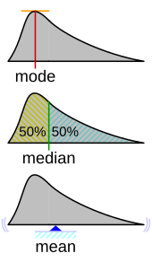
In symmetric unimodal distributions, such as the normal distribution, the mean (if defined), median and mode all coincide. For samples, if it is known that they are drawn from a symmetric unimodal distribution, the sample mean can be used as an estimate of the population mode.
YouTube Encyclopedic
-
1/5Views:232 1361 550 06415 14187 728490 845
-
Statistics - Find the mode for a set of data
-
Mean, Median, and Mode of Grouped Data & Frequency Distribution Tables Statistics
-
Calculate Mode from Continuous Group Data Statistics 10
-
Mode - Statistics
-
Statistics mode
Transcription
Mode of a sample
The mode of a sample is the element that occurs most often in the collection. For example, the mode of the sample [1, 3, 6, 6, 6, 6, 7, 7, 12, 12, 17] is 6. Given the list of data [1, 1, 2, 4, 4] its mode is not unique. A dataset, in such a case, is said to be bimodal, while a set with more than two modes may be described as multimodal.
For a sample from a continuous distribution, such as [0.935..., 1.211..., 2.430..., 3.668..., 3.874...], the concept is unusable in its raw form, since no two values will be exactly the same, so each value will occur precisely once. In order to estimate the mode of the underlying distribution, the usual practice is to discretize the data by assigning frequency values to intervals of equal distance, as for making a histogram, effectively replacing the values by the midpoints of the intervals they are assigned to. The mode is then the value where the histogram reaches its peak. For small or middle-sized samples the outcome of this procedure is sensitive to the choice of interval width if chosen too narrow or too wide; typically one should have a sizable fraction of the data concentrated in a relatively small number of intervals (5 to 10), while the fraction of the data falling outside these intervals is also sizable. An alternate approach is kernel density estimation, which essentially blurs point samples to produce a continuous estimate of the probability density function which can provide an estimate of the mode.
The following MATLAB (or Octave) code example computes the mode of a sample:
X = sort(x);                               % x is a column vector dataset
indices   =  find(diff([X; realmax]) > 0); % indices where repeated values change
[modeL,i] =  max (diff([0; indices]));     % longest persistence length of repeated values
mode      =  X(indices(i));
The algorithm requires as a first step to sort the sample in ascending order. It then computes the discrete derivative of the sorted list and finds the indices where this derivative is positive. Next it computes the discrete derivative of this set of indices, locating the maximum of this derivative of indices, and finally evaluates the sorted sample at the point where that maximum occurs, which corresponds to the last member of the stretch of repeated values.
Comparison of mean, median and mode
| Type | Description | Example | Result |
|---|---|---|---|
| Arithmetic mean | Sum of values of a data set divided by number of values | (1+2+2+3+4+7+9) / 7 | 4 |
| Median | Middle value separating the greater and lesser halves of a data set | 1, 2, 2, 3, 4, 7, 9 | 3 |
| Mode | Most frequent value in a data set | 1, 2, 2, 3, 4, 7, 9 | 2 |
Use
Unlike mean and median, the concept of mode also makes sense for "nominal data" (i.e., not consisting of numerical values in the case of mean, or even of ordered values in the case of median). For example, taking a sample of Korean family names, one might find that "Kim" occurs more often than any other name. Then "Kim" would be the mode of the sample. In any voting system where a plurality determines victory, a single modal value determines the victor, while a multi-modal outcome would require some tie-breaking procedure to take place.
Unlike median, the concept of mode makes sense for any random variable assuming values from a vector space, including the real numbers (a one-dimensional vector space) and the integers (which can be considered embedded in the reals). For example, a distribution of points in the plane will typically have a mean and a mode, but the concept of median does not apply. The median makes sense when there is a linear order on the possible values. Generalizations of the concept of median to higher-dimensional spaces are the geometric median and the centerpoint.
Uniqueness and definedness
For some probability distributions, the expected value may be infinite or undefined, but if defined, it is unique. The mean of a (finite) sample is always defined. The median is the value such that the fractions not exceeding it and not falling below it are each at least 1/2. It is not necessarily unique, but never infinite or totally undefined. For a data sample it is the "halfway" value when the list of values is ordered in increasing value, where usually for a list of even length the numerical average is taken of the two values closest to "halfway". Finally, as said before, the mode is not necessarily unique. Certain pathological distributions (for example, the Cantor distribution) have no defined mode at all.[citation needed][4] For a finite data sample, the mode is one (or more) of the values in the sample.
Properties
Assuming definedness, and for simplicity uniqueness, the following are some of the most interesting properties.
- All three measures have the following property: If the random variable (or each value from the sample) is subjected to the linear or affine transformation, which replaces X by aX + b, so are the mean, median and mode.
- Except for extremely small samples, the mode is insensitive to "outliers" (such as occasional, rare, false experimental readings). The median is also very robust in the presence of outliers, while the mean is rather sensitive.
- In continuous unimodal distributions the median often lies between the mean and the mode, about one third of the way going from mean to mode. In a formula, median ≈ (2 × mean + mode)/3. This rule, due to Karl Pearson, often applies to slightly non-symmetric distributions that resemble a normal distribution, but it is not always true and in general the three statistics can appear in any order.[5][6]
- For unimodal distributions, the mode is within √3 standard deviations of the mean, and the root mean square deviation about the mode is between the standard deviation and twice the standard deviation.[7]
Example for a skewed distribution
An example of a skewed distribution is personal wealth: Few people are very rich, but among those some are extremely rich. However, many are rather poor.
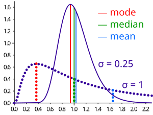
A well-known class of distributions that can be arbitrarily skewed is given by the log-normal distribution. It is obtained by transforming a random variable X having a normal distribution into random variable Y = eX. Then the logarithm of random variable Y is normally distributed, hence the name.
Taking the mean μ of X to be 0, the median of Y will be 1, independent of the standard deviation σ of X. This is so because X has a symmetric distribution, so its median is also 0. The transformation from X to Y is monotonic, and so we find the median e0 = 1 for Y.
When X has standard deviation σ = 0.25, the distribution of Y is weakly skewed. Using formulas for the log-normal distribution, we find:

Indeed, the median is about one third on the way from mean to mode.
When X has a larger standard deviation, σ = 1, the distribution of Y is strongly skewed. Now

Here, Pearson's rule of thumb fails.
Van Zwet condition
Van Zwet derived an inequality which provides sufficient conditions for this inequality to hold.[8] The inequality
- Mode ≤ Median ≤ Mean
holds if
- F( Median - x ) + F( Median + x ) ≥ 1
for all x where F() is the cumulative distribution function of the distribution.
Unimodal distributions
It can be shown for a unimodal distribution that the median and the mean lie within (3/5)1/2 ≈ 0.7746 standard deviations of each other.[9] In symbols,


where is the absolute value.

A similar relation holds between the median and the mode: they lie within 31/2 ≈ 1.732 standard deviations of each other:

History
The term mode originates with Karl Pearson in 1895.[10]
Pearson uses the term mode interchangeably with maximum-ordinate. In a footnote he says, "I have found it convenient to use the term mode for the abscissa corresponding to the ordinate of maximum frequency."
See also
- Arg max
- Central tendency
- Descriptive statistics
- Moment (mathematics)
- Summary statistics
- Unimodal function
References
- ^ Damodar N. Gujarati. Essentials of Econometrics. McGraw-Hill Irwin. 3rd edition, 2006: p. 110.
- ^ Zhang, C; Mapes, BE; Soden, BJ (2003). "Bimodality in tropical water vapour". Q. J. R. Meteorol. Soc. 129 (594): 2847–2866. Bibcode:2003QJRMS.129.2847Z. doi:10.1256/qj.02.166. S2CID 17153773.
- ^ "AP Statistics Review - Density Curves and the Normal Distributions". Archived from the original on 2 April 2015. Retrieved 16 March 2015.
- ^ Morrison, Kent (1998-07-23). "Random Walks with Decreasing Steps" (PDF). Department of Mathematics, California Polytechnic State University. Archived from the original (PDF) on 2015-12-02. Retrieved 2007-02-16.
- ^ "Relationship between the mean, median, mode, and standard deviation in a unimodal distribution".
- ^ Hippel, Paul T. von (2005). "Mean, Median, and Skew: Correcting a Textbook Rule". Journal of Statistics Education. 13 (2). doi:10.1080/10691898.2005.11910556.
- ^ Bottomley, H. (2004). "Maximum distance between the mode and the mean of a unimodal distribution" (PDF). Unpublished Preprint.
- ^ van Zwet, WR (1979). "Mean, median, mode II". Statistica Neerlandica. 33 (1): 1–5. doi:10.1111/j.1467-9574.1979.tb00657.x.
- ^ Basu, Sanjib; Dasgupta, Anirban (1997). "The mean, median, and mode of unimodal distributions: a characterization". Theory of Probability & Its Applications. 41 (2): 210–223. doi:10.1137/S0040585X97975447.
- ^ Pearson, Karl (1895). "Contributions to the Mathematical Theory of Evolution. II. Skew Variation in Homogeneous Material". Philosophical Transactions of the Royal Society of London A. 186: 343–414. Bibcode:1895RSPTA.186..343P. doi:10.1098/rsta.1895.0010.
External links
- "Mode", Encyclopedia of Mathematics, EMS Press, 2001 [1994]
- A Guide to Understanding & Calculating the Mode
- Weisstein, Eric W. "Mode". MathWorld.
- Mean, Median and Mode short beginner video from Khan Academy