


In probability theory and directional statistics, a wrapped exponential distribution is a wrapped probability distribution that results from the "wrapping" of the exponential distribution around the unit circle.
YouTube Encyclopedic
-
1/5Views:19 8851 60683846415 666
-
4. Poisson (the Perfect Arrival Process)
-
Karl T. Ulrich "The Importance of the Raw Idea in Innovation; Testing the Sow's Ear Hypothesis"
-
3g Stability of the MHD equilibrium
-
Karatbars Marketing Tool
-
Lec 22 | MIT 3.091SC Introduction to Solid State Chemistry, Fall 2010
Transcription
The following content is provided under a Creative Commons license. Your support will help MIT OpenCourseWare continue to offer high quality educational resources for free. To make a donation or view additional materials from hundreds of MIT courses, visit MIT OpenCourseWare at ocw.mit.edu. PROFESSOR: As the question said, where are we as far as the text goes. We're just going to start Chapter 2 today, Poisson processes. I want to spend about five minutes reviewing a little bit about convergence, the things we said last time, and then move on. There's a big break in the course, at this point between Chapter 1 and Chapter 2 in the sense that Chapter 1 is very abstract, a little theoretical. It's dealing with probability theory in general and the most general theorems in probability stated in very simple and elementary form. But still, we're essentially not dealing with applications at all. We're dealing with very, very abstract things in Chapter 1. Chapter 2 is just the reverse. A Poisson process is the most concrete thing you can think of. People use that as a model for almost everything. Whether it's a reasonable model or not is another question. But people use it as a model constantly. And everything about it is simple. For a Poisson process, you can almost characterize it as saying everything you could think of about a Poisson process is either true or it's obviously false. And when you get to that point, you understand Poisson processes. And you can go on to other things and never have to really think about them very hard again. Because at that point, you really understand them. OK. So let's go on and review things a little bit. What's convergence and how does it affect sequences of IID random variables? Convergence is more general than just IID random variables. But it applies to any sequence of random variables. And the definition is that a sequence of random variables converges in distribution to another random variable z, if the limit, as n goes to infinity, of the distribution function of zn converges to the distribution function of z. For this definition to make sense, it doesn't matter what z is. z can be outside of the sample space even. The only thing we're interested in is this particular distribution function. So what we're really saying is a sequence of distributions converges to another distribution function if in fact this limit occurs at every point where f of z is continuous. In other words, if f of z is discontinuous someplace, we had an example of that where we're looking at the law of large numbers and the distribution function. Looked at in the right way was a step function. It wasn't continuous at the step. And therefore, you can't expect anything to be said about that. So the typical example of convergence in distribution is the central limit theorem which says, if x1, x2 are IID, they have a variance sigma squared. And if s sub n the sum of these random variables is a sum of x1 to xn, then zn is the normalized sum. In other words, you take this sum. You subtract off the mean of it. And I think in the reproduction of these slides that you have, I think that n, right there was-- here we go. That's the other y. I think that n was left off. If that n wasn't left off, another n was left off. It's obviously needed there. This is a normalized random variable because the variance of sn and of sn minus nx bar is just sigma squared times n. Because they're any of these random variables. So we're dividing by the standard deviation. So this is a random variable for each n which has a standard deviation 1 and mean 0. So it's normalized. And it converges in distribution to a Gaussian random variable of mean 0 and standard deviation 1. This notation here is sort of standard. And we'll use it at various times. It means a Gaussian distribution with mean 0 and variance 1. So for an example of that, if x1, x2, so forth, are IID with mean expected value of x and the sum here, then sn over n converges in distribution to the deterministic random variable x bar. That's a nice example of this. So we have two examples of convergence and distribution. And that's what that says. So next, a sequence of random variables converges in probability. When we start talking about convergence in probability, there's another idea which we are going to bring in, mostly in Chapter 4 when we get to it, which is called convergence with probability 1. Don't confuse those two things because they're very different ideas. Because people confuse them, many people call convergence with probability 1 almost sure convergence or almost everywhere convergence. I don't like that notation. So I'll stay with the notation with probability 1. But it means something very different than converging in probability. So the definition is that a set of random variables converges in probability to some other random variable if this limit holds true. And you remember that diagram we showed you last time. Let me just quickly redraw it. Have this set of distribution functions. Here's the mean here, x bar, limits, plus and minus epsilon. And this sequence of random variables has to come in down here and go out up there. This distance here and the distance there gets very small and goes to 0 as n gets very large. And that's the meaning of what this says. So if you don't remember that diagram, go look at it in the lecture notes last time or in the text where it's explained in a lot more detail. So the typical example of that is the weak law of large numbers of x1, blah, blah, blah, are IID with mean, expected value of x. Remember now that we say that a random variable has a mean if the expected value of the absolute value of x is finite. It's not enough to have things which have a distribution function which is badly behaved for very big x, and badly behaved for very small x, and the two of them cancelled out. That doesn't work. That doesn't mean you have a mean. You need the expected value as the absolute value of x to be finite. Now, the weak law of large numbers says that the random variables sn over n, in other words, the sample average, in fact converges to the deterministic random variable x bar. And that convergence is convergence in probability. Which means it's this kind of convergence here. Which means that it's going to a distribution which is a step function. There's a very big difference between a distribution which is a step function and a distribution which is something like a Gaussian random variable. And what the big difference is is that the random variables that are converging to each other, if a bunch of random variables are all converging to a constant, then they all have to be very close to each other. And that's the property you're really interested in in convergence in probability. So convergence in mean square, finally, last definition which is easy to deal with. If a sequence of random variables converges in the mean square to another random variable, if this limit of the expected value, of the difference between the two random variables squared, goes to 0, this n gets big. That's what we had with the weak law of large numbers if you assume that the random variables each had a variance. So on to something new. On to Poisson processes. We first have to explain what an arrival process is. And then we can get into Poisson processes. Because arrival processes are a very broad class of stochastic processes, in fact discrete stochastic processes. But they have this property of being characterized by things happening at various random instance of time as opposed to a noise waveform or something of that sort. So an arrival process is a sequence of increasing random variables, 0 less than s1, less than s2. What's it mean for a random variable s1 to be less than a random variable s2? It means exactly the same thing as it means for real numbers. s1 is less than s2 if the random variable s2 minus s1 is a positive random variable, namely if it only takes on non-negative values for all omega in the sample space or for all omega except for some peculiar set of probability 0. The differences in these arrival epochs, why do I call them arrival epochs? Why do other people call them arrival epochs? Because time is something which gets used so often here that it gets confusing. So it's nice to call one thing epochs instead of time. And then you know what you're talking about a little better. The difference is s sub i minus s sub i minus 1 for all i greater than or equal to 2 here, with x1 equal to s1. These are called interarrival times and the si are called arrival epochs. The picture here really shows it all. Here we have a sequence of arrival instance, which is where these arrivals occur. By definition, x1 is the time at which is the first arrival occurs, x2 is the difference between the time when the second arrival occurs and the first arrival occurs, and so forth. n of t is the number of arrivals that have occurred up until time t. Which is, if we draw a staircase function for each of these arrivals, n of t is just the value of that staircase function. In other words, the counting process, the arrival counting process-- here's another typo in the notes that you've got. It calls it Poisson counting process. It should be arrival counting process. What this staircase function is is in fact the counting process. It says how many arrivals there have been up until time t. And every once in a while, that jumps up by 1. So it keeps increasing by 1 at various times. So that's the arrival counting process. The important thing to get out of this is if you understand everything about these random variables, then you understand everything about these random variables. And then you understand everything about these random variables. There's a countable number of these random variables. There's a countable number of these random variables. There's an unaccountably infinite number of these random variables. In other words, for every t, n of t is a different random variable. I mean, it tends to be the same for relatively large intervals of t sometimes. But this is a different random variable for each value of t. So let's proceed with that. A sample path or sample function of the process is a sequence of sample values. That's the same as we have everywhere. You look at a sample point of the process. Sample point of the whole probability space maps into this sequence of random variables, s1, s2, s3, and so forth. If you know what the sample value is of each one of these random variables, then in fact, you can draw this step function here. If you know the value, the sample value, of each one of these, in the same way, you can again draw this step function. And if you know what the subfunction is, the step function in fact is the sample value of n of t. Now, there's one thing a little peculiar here. Each sample path corresponds to a particular staircase function. And the process can be viewed as the ensemble with joint probability distributions of such staircase functions. Now, what does all that gobbledygook mean? Very, very often in probability theory, we draw pictures. And these pictures are pictures of what happens to random variables. And there's a cheat in all of that. And the cheat here is that in fact, this step function here is just a generic step function. These points at which changes occur are generic values at which changes occur. And we're representing those values as random variables. When you represent these as random variables, this whole function here, namely n of t itself, becomes-- if you have a particular set of values for each one of these, then you have a particular staircase function. With that particular staircase function, you have a particular sample path for n of t. In other words, a sample path for any set of these random variables-- the arrival epochs, or the interarrival intervals, or n of t for each t-- all of these are equivalent to each other. For this reason, when we talk about arrival processes, it's a little different than what we usually do. Because usually, we say a random process is a sequence or an uncountable number of random variables. Here, just because we can describe it in three different ways, this same stochastic process gets described either as a sequence of interarrival intervals, or as a sequence of arrival epochs, or as a countable number these n of t random variables. And from now on, we make no distinction between any of these things. We will, every once in while, have to remind ourselves what these pictures mean because they look very simple. They look like the pictures of functions that you're used to drawing. But they don't really mean the same thing. Because this picture is drawing a generic sample path. For that generic sample path, you have a set of sample values for the Xs, a sample path for the arrival epochs, a sample set of values for n of t. And when we draw the picture calling these random variables, we really mean the set of all such step functions. And we just automatically use all those properties and those relationships. So it's not quite as simple as what it appears to be, but it's almost as simple. You can also see that any sample path can be specified by the sample values n of t for all t, by si for all i, or by xi for all i. So that essentially, an arrival process is specified by any one of these things. That's exactly what I just said. The major relation we need to relate the counting process to the arrival process, well, there's one relationship here, which is perhaps the simplest relationship. But this relationship is a nice relationship to say what n of t is if you know what s sub n is. It's not quite so nice if you know what n of t is to figure what s sub n is. I mean, the information is tucked into the statement, but it's tucked in a more convenient way into this statement down here. This statement, I can see it now after many years of dealing with it. I'm sure that you can see it if you stare at it for five minutes. You will keep forgetting the intuitive picture that goes with it. So I suggest that this is one of the rare things in this course that you just ought to remember. And then once you remember it, you can always figure out why it's true. Here's the reason why it's true. If s sub n is equal to tau for some tau less than or equal to t, then n of tau has to be equal to n. If s sub n is equal to tau, here's the picture here, except there's not a tau here. If s sub 2 is equal to tau, then n of 2-- these are right continuous, so n of 2 is equal to 2. And therefore, n of tau is less than or equal to n of t. So that's the whole reason down there. You can turn this argument around. You can start out with n of t is greater than or equal to n. It means n of t is equal to some particular n. And turn the argument upside down. And you get the same argument. So this tells you what this is. This tells you what this is. If you do this for every n and every t, then you do this for every n and every t. It's a very bizarre statement because usually when you have relationships between functions, you don't have the Ns and the Ts switching around. And in this case, the n is the subscript. That's the thing which says which random variable you're talking about. And over here, t is the thing which says what random variable you're talking about. So it's peculiar in that sense. It's a statement which requires a little bit of thought. I apologize for dwelling on it because once you see it, it's obvious. But many of these obvious things are not obvious. What we're going to do as we move on is we're going to talk about these arrival processes in any of these three ways we choose to talk about them. And we're going to go back and forth between them. And with Poisson processes, that's particularly easy. We can't do a whole lot more with arrival processes. They're just too complicated. I mean, arrival processes involve almost any kind of thing where things happen at various points in time. So we simplify it to something called a renewal process. Renewal processes are the topic of Chapter 4. When you get to Chapter 4, you will perhaps say that renewal processes are too complicated to talk about also. I hope after we finish Chapter 4, you won't believe that it's too complicated to talk about. But these are fairly complicated processes. But even here, it's an arrival process where the interarrival intervals are independent and identically distributed. Finally, a Poisson process is a renewal process for which each x sub i has an exponential distribution. Each interarrival has to have the same distribution because since it's a renewal process, these are all IID. And we let this distribution function X be the generic random variable. And this is talking about the distribution function of all of them. I don't know whether that 1 minus is in the slides I passed out. There's one kind of error like that. And I'm not sure where it is. So anyway, lambda is some fixed parameter called the rate of the Poisson process. So for each lambda greater than 0, you have a Poisson process where each of these interarrival intervals are exponential random variables of rate lambda. So that defines a Poisson process. So we can all go home now because we now know everything about Poisson processes in principle. Everything we're going to say from now on comes from this one simple statement here that these interarrival intervals are exponential. There's something very, very special about this exponential distribution. And that's what makes Poisson processes so very special. And that special thing is this memoryless property. A random variable is memoryless if it's positive. And for all real t greater than 0 and x greater than 0, the probability that x is greater than t plus x is equal to the probability that x is greater than t times the probability that x is greater than x. If you plug that in, then the statement is the same whether you're dealing with densities, or PMFs, or distribution function. You get the same product relationship in each case. Since the interarrival interval is exponential, the probability that a random variable x is greater than some particular value x is equal to e to the minus lambda x for x greater than zero. This you'll recognize, not as a distribution function but as the complementary distribution function. It's the probability that X is greater than x. So it's the complementary distribution function evaluated at the value of x. This is an exponential which is going down. So these random variables have a probability density which is this. This is f sub x of X. And they have a distribution function which is this. And they have a complementary distribution function which is this. Now, this is f of c. This is f. So there's nothing much to them. And now there's a theorem which says that a random variable is memoryless if and only if it is exponential. We just showed here that an exponential random variable is memoryless. To show it the other way is almost obvious. You take this definition here. You take the logarithm of each of these sides. When you get the logarithm of this, it says the logarithm of the probability x is greater than p plus x is the logarithm of this plus the logarithm of this. What we have to show to get an exponential is that this logarithm is linear in its argument t. Now, if you have this is equal to the sum of this and this for all t and x, it's sort of says it's linear. There's an exercise, I think it's Exercise 2.4, which shows that you have to be a little bit careful. Or at least as it points out, very, very picky mathematicians have to be a little bit careful with that. And you can worry about that or not as you choose. So that's the theorem. That's why Poisson processes are special. And that's why we can do all the things we can do with them. The reason why we call it memoryless is more apparent if we use conditional probabilities. With conditional probabilities, the probability that the random variable X is greater than t plus x, given that it's greater than t, is equal to the probability that X is greater than x. If people in a checkout line have exponential service times and you've waited 15 minutes for the person in front, what is his or her remaining service time, assuming the service time is exponential? What's the answer? You've waited 15 minutes. Your original service time is exponential with rate lambda. What's the remaining service time? Well, the answer is it's exponential. That's this memoryless property. It's called memoryless because the random variable doesn't remember how long it hasn't happened. So you can think of an exponential random variable as something which takes place in time. And in each instant of time, it might or might not happen. And if it hasn't happened yet, there's still the same probability in every remaining increment that it's going to happen then. So you haven't gained anything and you haven't lost anything by having to wait this long. Here's an interesting question which you can tie yourself in knots for a little bit. Has your time waiting been wasted? Namely the time you still have to wait is exponential with the same rate as it was before. So the expected amount of time you have to wait is still the same as when you got into line 15 minutes ago with this one very slow person in front of you. So have you wasting your time? Well, you haven't gained anything. But you haven't really wasted your time either. Because if you have to get served in that line, then at some point, you're going to have to go in that line. And you might look for a time when the line is very short. You might be lucky and find a time when the line is completely empty. And then you start getting served right away. But if you ignore those issues, then in fact, in a sense, you have wasted your time. Another more interesting question then is why do you move to another line if somebody takes a long time? All of you have had this experience. You're in a supermarket. Or you're at an airplane counter or any of the places where you have to wait for service. There's somebody, one person in front of you, who has been there forever. And it seems as if they're going to stay there forever. You notice another line that only has one person being served. And most of us, especially very impatient people like me, I'm going to walk over and get into that other line. And the question is, is that rational or isn't it rational? If the service times are exponential, it is not rational. It doesn't make any difference whether I stay where I am or go to the other line. If the service times are fixed duration, namely suppose every service time takes 10 minutes and I've waited for a long time, is it rational for me to move to the other line? Absolutely not because I'm almost at the end of that 10 minutes now. And I'm about to be served. So why do we move? Is it just psychology, that we're very impatient? I don't think so. I think it's because we have all seen that an awful lot of lines, particularly airline reservation lines, and if your plane doesn't fly or something, and you're trying to get rescheduled, or any of these things, the service time is worse than Poisson in the sense that if you've waited for 10 minutes, your expected remaining waiting time is greater than it was before you started waiting. The longer you wait, the longer your expected remaining waiting time is. And that's called a heavy-tailed distribution. What most of us have noticed, I think, in our lives is that an awful lot of waiting lines that human beings wait in are in fact heavy-tailed. So that in fact is part of the reason why we move if somebody takes a long time. It's interesting to see how the brain works. Because I'm sure that none of you have ever really rationally analyzed this question of why you move. Have you? I mean, I have because I teach probability courses all the time. But I don't think anyone who doesn't teach probability courses would be crazy enough to waste their time on a question like this. But your brain automatically figures that out. I mean, your brain is smart enough to know that if you've waited for a long time, you're probably going to have to wait for an even longer time. And it makes sense to move to another line where your waiting time is probably going to be shorter. So you're pretty smart if you don't think about it too much. Here's an interesting theorem now that makes use of this memoryless property. This is Theorem 2.2.1 in the text. It's not stated terribly well there. And I'll tell you why in a little bit. It's not stated too badly. I mean, it's stated correctly. But it's just a little hard to understand what it says. If you have a Poisson process of rate lambda and you're looking at any given time t, here's t down here. You're looking at the process of time t. The interval z-- here's the interval z here-- from t until the next arrival has distribution e to the minus lambda z. And it has this distribution for all real numbers greater than 0. The random variable Z is independent of n of t. In other words, this random variable here is independent of how many arrivals there have been at time t. And given this, it's independent of s sub n, which is the time at which the last arrival occurred. Namely, here's n of t equals 2. Here's s of 2 at time tau. So given both n of t and s sub 2 in this case, or s sub n of t as we might call it, and that's what gets confusing. And I'll talk about that later. Given those two things, the number n of arrivals in 0t-- well, I got off. The random variable Z is independent of n of t. And given n of t, Z is independent of all of these arrival epochs up until time t. And it's also independent of n of t for all values of tau up until t. That's what the theorem states. What the theorem states is that this memoryless property that we've just stated for random variables is really a property of the Poisson process. When we say that if a random variable, it's a little hard to see why would anyone was calling it memoryless. When you state it for a Poisson process, it's very obvious why we want to call it memoryless. It says that this time here from t, from any arbitrary t, until the next arrival occurs, that this is independent of all this junk that happens before or up to time t. That's what the theorem says. Here's a sort of a half proof of it. There's a careful proof in the notes. The statement in the notes is not that careful, but the proof is. And the proof is drawn out perhaps too much. You can find your comfort level between this and the much longer version in the notes. You might understand it well from this. Given n of t is equal to 2 in this case, and in general, given that n of t is equal to any constant n, and given that s sub 2 where this 2 is equal to that 2, given that s sub 2 is equal to tau, then x3, this value here, the interarrival arrival time from this previous arrival before t to the next arrival after t, namely x3, is the thing which bridges across this time that we selected, t. t is not a random thing. t is just something you're interested in. I want to catch a plane at 7 o'clock tomorrow evening. t then is 7 o'clock tomorrow evening. What's the time from the last plane that went out to New York until the next plane that's going out to New York? If the planes are so screwed up that the schedule means nothing, then they're just flying out whenever they can fly out. That's the meaning of this x3 here. That says that x3, in fact, has to be bigger than t minus tau. If we're given that n of t is equal to 2 and that the time of the previous arrival is at tau, we're given that there haven't been any arrivals between the last arrival before t and t. That's what we're given. This was the last arrival before t by the assumption we've made. So we're assuming there's nothing in this interval. And then we're asking what is the remaining time until x3 is all finished. And that's the random variable that we call Z. So Z is x3 minus t minus tau. The complementary distribution function of Z conditional on both n and on s, this n here and this s here is then exponential with e to the minus lambda Z. Now, if I know that this is exponential, what can I say about the random variable Z itself? Well, there's an easy way to find the distribution of Z when you know Z conditional onto other things. You take what the distribution is conditional on, each value of n and s. You then multiply that by the probability that n and s have those particular values. And then you integrate. Now, we can look at this and say we don't have to go through all of that. And in fact, we won't know what the distribution of n is. And we certainly won't know what the distribution of this previous arrival is for quite a long time. Why don't we need to know that? Well, because we know that whatever n of t is and whatever s sub n of t is doesn't make any difference. The distribution of Z is still the same thing. So we know this has to be the unconditional distribution function of Z also even without knowing anything about n or knowing about s. And that means that the complementary distribution function of Z is equal to e to the minus lambda Z also. So that's sort of a proof if you want to be really picky. And I would suggest you try to be picky. When you read the notes, try to understand why one has to say a little more than one says here. Because that's the way you really understand these things. But this really gives you the idea of the proof. And it's pretty close to a complete proof. This is saying what we just said. The conditional distribution of Z doesn't vary with the conditioning values. n of t equals n. And s sub n equals tau. So Z is statistically independent of n of t and s sub n of t. You should look at the text again, as I said, for more careful proof of that. What is this random variable s sub n of t? It's clear from the picture what it is. s sub n of t is the last arrival before we're at time t. That's what it is in the picture here. How do you define a random variable like that? There's a temptation to do it the following way which is incorrect. There's a temptation to say, well, conditional on n of t, suppose n of t is equal to n. Let me then find the distribution of s sub n. And that's not the right way to do it. Because s sub n of t and n of t are certainly not independent. n of t tells you what random variable you want to look at. How do you define a random variable in terms of a mapping from the sample space omega onto the set of real numbers? So what you do here is you look at a sample point omega. It maps into this random variable n of t, the sample value of that at omega, that's sum value n. And then you map that same sample point into-- now, you know which random variable it is you're looking at. You take that same omega and map it into sub time tau. So that's what we mean by s sub n of t. If your mind glazes over at that, don't worry about it. Think about it a little bit now. Come back and think about it later. Every time I don't think about this for two weeks, my mind glazes over when I look at it. And I have to think very hard about what this very peculiar looking random variable is. When I have a random variable where I have a sequence of random variables, and I have a random variable which is a random selection among those random variables, it's a very complicated animal. And that's what this is. But we've just said what it is. So you can think about it as you go. The theorem essentially extends the idea of memorylessness to the entire Poisson process. In other words, this says that a Poisson process is memoryless. You look at a particular time t. And the time until the next arrival is independent of everything that's going before that. Starting at any time tau, yeah, well, subsequent interrarrival times are independent of Z and also of the past. I'm waving my hands a little bit here. But in fact, what I'm saying is right. We have these interarrival intervals that we know are independent. The interarrival intervals which have occurred completely before time t are independent of this random variable Z. The next interarrival interval after Z is independent of all the interarrival intervals before that. And those interarrival intervals before that are determined by the counting process up until time t. So the counting process corresponds to this corresponding interarrival process. It's n of t prime minus n of t for t prime greater than t. In other words, we now want to look at a counting process which starts at time t and follows whatever it has to follow from this original counting process. And what we're saying is this first arrival and this process starting at time t is independent of everything that went before. And every subsequent interarrival time after that is independent of everything before time t. So this says that the process n of t prime minus n of t as a process nt prime. This is a counting process nt prime defined for t prime greater than t. So for fixed t, we now have something which we can view over variable t prime as a counting process. It's a Poisson process shifted to start at time t, ie, for each t prime, n of t prime minus the n of t has the same distribution as n of t prime minus t. Same for joint distributions. In other words, this random variable Z is exponential again. And all the future interarrival times are exponential. So it's defined in exactly the same way as the original random process is. So it's statistically the same process. Which says two things about it. Everything is the same. And everything is independent. We will call that stationary. Everything is the same. And independent, everything is independent. And then we'll try to sort out how things can be the same but also be independent. Oh, we already know that. We have two IID random variables, x1 and x2. They're IID. They're independent and identically distributed. Identity distributed means that in one sense, they are the same. But they're also independent of each other. So the random variables are defined in the same way. And in that sense, they're stationary. But they're independent of each other by the definition of independence. So our new process is independent of the old process in the interval 0 up to t. When we're talking about Poisson processes and also arrival processes, we always talk about intervals which are open on the left and closed on the right. That's completely arbitrary. But if you don't make one convention or the other, you could make them closed on the left and open on the right, and that would be consistent also. But nobody does. And it would be much more confusing. So it's much easier to make things closed on the right. So we're up to stationary and independent increments. Well, we're not up to there. We're almost finished with that. We've virtually already said that increments are stationary and independent. And an increment is just a piece of a Poisson process. That's an increment, a piece of it. So a counting process has the stationary increment property if n of t prime minus n of t has the same distribution as n of t prime minus t for all t prime greater than t greater than 0. In other words, you look at this counting process. Goes up. Then you start at some particular value of t. Let me draw a picture of that. Make it a little clearer. And the new Poisson process starts at this value and goes up from there. So this thing here is what we call n of t prime minus n of t. Because here's n of t. Here's t prime out here for any value out here. And we're looking at the number of arrivals up until time t prime. And what we're talking about, when we're talking about n of t prime minus n of t, we're talking about what happens in this region here. And we're saying that this is a Poisson process again. And now in a minute, we're going to say that this Poisson process is independent of what happened up until time t. But Poisson processes have this stationary increment property. And a counting process has the independent increment property if for every sequence of times, t1, t2, up to t sub n. The random variables n of t1 and tilde of t1, t2, we didn't talk about that. But I think it's defined on one of those slides. n of t and t prime is defined as n of t prime minus n of t. So n of t and t prime is really the number of arrivals that have occurred from t up until t prime-- open on t, closed on t prime. So a counting process has the independent increment property if for every finite set of times, these random variables here are independent. The number of arrivals in the first increment, number of arrivals in the second increment, number of arrivals in the third increment, no matter how you choose t1, t2, up to t sub n, what happens here is independent of what happens here, is independent of what happens here, and so forth. It's not only that what happens in Las Vegas stays there. It's that what happens in Boston stays there, what happens in Philadelphia stays there, and so forth. What happens anywhere stays anywhere. It never gets out of there. That's what we mean by independence in this case. So it's a strong statement. But we've essentially said that Poisson processes have that property. So this property implies is the number of arrivals in each of the set of non-overlapping intervals are independent random variables. For a Poisson process, we've seen that the number of arrivals in t sub i minus 1 to t sub i is independent of this whole set of random variables here. Now, remember that when we're talking about multiple random variables, we say that multiple random variables are independent. It's not enough to be pairwise independent. They all have to be independent. But this thing we've just said says that this is independent of all of these things. If this is independent of all of these things, and then the next interval n of ti, ti plus 1, is independent of everything in the past, and so forth all the way up, then all of those random variables are statistically independent of each other. So in fact, we're saying more than pairwise statistical independence. If you're panicking about these minor differences between pairwise independence and real independence, don't worry about it too much. Because the situations where that happens are relatively rare. They don't happen all the time. But they do happen occasionally. So you should be aware of it. You shouldn't get in a panic about it. Because normally, you don't have to worry about it. In other words, when you're taking a quiz, don't worry about any of the fine points. Figure out roughly how to do the problems. Do them more or less. And then come back and deal with the fine points later. Don't spend the whole quiz time wrapped up on one little fine point and not get to anything else. One of the important things to learn in understanding a subject like this is to figure out what are the fine points, what are the important points. How do you tell whether something is important in a particular context. And that just takes intuition. That takes some intuition from working with these processes. And you pick that up as you go. But anyway, we wind up now with the statement that Poisson processes have stationary and independent increments. Which means that what happens in each interval is independent of what happens in each other interval. So we're done with that until we get to alternate definitions of a Poisson process. And we now want to deal with the Erlang and the Poisson distributions, which are just very plug and chug kinds of things to a certain extent. For a Poisson process of rate lambda, the density function of arrival epoch s2, s2 is the sum of x1 plus x2. x1 is an exponential random variable of rate lambda. x2 is an independent random variable of rate lambda. How do you find the probability density function as a sum of two independent random variables, which both have a density? You convolve them. That's something that you've known ever since you studied any kind of linear systems, or from any probability, or anything else. Convolution is the way to solve this problem. When you convolve these two random variables, here I've done it. You get lambda squared t times e to the minus lambda t. This kind of form here with an e to the minus lambda t, and with a t, or t squared, or so forth, is a particularly easy form to integrate. So we just do this again and again. And when we do it again and again, we find out that the density function as a sum of n of these random variables, you keep picking up an extra lambda every time you convolve in another exponential random variable. You pick up an extra factor of t whenever you do this again. This stays the same as it does here. And strangely enough, this n minus 1 factorial appears down here when you start integrating something with some power of t in it. So when you integrate this, this is what you get. And it's called the Erlang density. Any questions about this? Or any questions about anything? I'm getting hoarse. I need questions. [LAUGHS] There's nothing much to worry about there. But now, we want to stop and smell the roses while doing all this computation. Let's do this a slightly different way. The joint density of x1 up to x sub n is lambda x1 times e to the minus lambda x1, times lambda x2, times e to the minus lambda x2, and so forth. So excuse me. The probability density of an exponential random variable is lambda times e to the minus lambda x. So the joint density is lambda e to the minus lambda x1. I told you I was getting hoarse. And my mind is getting hoarse. So you better start asking some questions or I will evolve into meaningless chatter. And this is just lambda to the n times e to the minus lambda times the summation of x sub i from i equals 1 to n. Now, that's sort of interesting because this joint density is just this simple-minded thing. You can write it as lambda to the n times e to the minus lambda s sub n, where s sub n is the time of the n-th arrival. This says that the joint distribution of all of these interarrival times only depends on when the last one comes in. And you can transform that to a joint density on each of the arrival epochs as lambda to the n times e to the minus lambda s sub n. Is this obvious to everyone? You're lying. If you're not shaking your head, you're lying. Because it's not obvious at all. What we're doing here, it's sort of obvious if you look at the picture. It's not obvious when you do the mathematics. What the picture says is-- let me see if I find the picture again. OK. Here's the picture up here. We're looking at these interarrival intervals. I think it'll be clearer if I draw it a different way. There we go. Let's just draw this in a line. Here's 0. Here's s1. Here's s2. Here's s3. And here's s4. And here's x1. Here's x2. Here's x3. And here's x4. Now, what we're talking about, we can go from the density of each of these intervals to the density of each of these sums in a fairly straightforward way. If you write this all out as a density, what you find is that in making a transformation from the density of these interarrival intervals to the density of these, what you're essentially doing is taking this density and multiplying it by a matrix. And the matrix is a diagonal matrix, is an upper triangular matrix. Because this depends only on this. This depends only on this and this. This depends only on this and this. This depends only on each of these. So it's a triangular matrix with terms on the diagonal. And when you look at a matrix like that, the terms on the diagonal are 1s because what's getting added each time is 1 times a new variable. So we have a matrix with 1s on the main diagonal and other stuff above that. And what that means is that when you make this transformation in densities, the determinant of that matrix is 1. And the value that you then get when you go from the density of these to the density of these, it's a uniform density again. So in fact, it has to look like what we said it looks like. So I was kidding you there. It's not so obvious how to do that although it looks reasonable. AUDIENCE: [INAUDIBLE]. PROFESSOR: Yeah. AUDIENCE: I'm sorry. Is it also valid to make an argument based on symmetry? PROFESSOR: It will be later. The symmetry is not clear here yet. I mean, the symmetry isn't clear because you're starting at time 0. And because you're starting at time 0, you don't have symmetry here yet. If we started at time 0 and we ended at some time t, we could try to claim there is some kind of symmetry between everything that happened in the middle. And we'll try to do that later. But at the moment, we would get into even more trouble if we try to do it by symmetry. But anyway, what this is saying is that this joint density is really-- if you know where this point is, the joint density of all of these things remains the same no matter how you move these things around. If I move s1 around a little bit, it means that x1 gets a little smaller, x2 gets a little bit bigger. And if you look at the joint density there, the joint density stays absolutely the same because you have e to the minus lambda x1 times e to the minus lambda x2. And the sum of the two for a fixed value here is the same as it was before. So you can move all of these things around in any way you want to. And the joint density depends only on the last one. And that's a very strange property and it's a very interesting property. And it sort of is the same as this independent increment property that we've been talking about. But we'll see why that is in just a minute. But anyway, once we have that property, we can then integrate this over the volume of s1, s2, s3, and s4, over that volume which has the property that it stops at that one particular point there. And we do that integration subject to the fact that s3 has to be less than or equal to s4, s2 has to be less than or equal to s3, and so forth down. When you do that integration, you get exactly the same thing as you got before when you did the integration. The integration that you did before was essentially doing this, if you look at what you did before. You were taking lambda times e to the minus lambda x times lambda times t minus x. And the x doesn't make any difference here. The x cancels out. That's exactly what's going on. And if you do it in terms of s1 and s2, the s1 cancels out. The s1 is the same as x here. So there is that cancellation here. And therefore, this Erlang density is just a marginal distribution of a very interesting joint distribution, which depends only on the last term. So next, we have a theorem which says for a Poisson process, the PMF for n of t, the Probability Mass Function, is the Poisson PMF. It sounds like I'm not really saying anything because what else would it be? Because you've always heard that the Poisson PMF is this particular function here. Well, in fact, there's some reason for that. And in fact, if we want to say that a Poisson process is defined in terms of these exponential interarrival times, then we have to show that this is consistent with that. The way I'll prove that here, this is a little more than a PF. Maybe we should say it's a P-R-O-F. Leave out the double O because it's not quite complete. But what we want to do is to calculate the probability that the n plus first arrival occurs sometime between t and t plus delta. And we'll do it in two different ways. And one way involves the probability mass function for the Poisson. The other way involves the Erlang density. And since we already know the Erlang density, we can use that to get the PMF for n of t. So using the Erlang density, the probability that the n plus first arrival falls in this little tiny interval here, we're thinking of delta as being small. And we're going to let delta approach 0. It's going to be the density of the n plus first arrival times delta plus o of delta. o of delta is something that goes to 0 as delta increases faster than delta does. It's something which has the property that o of delta divided by delta goes to 0 as delta gets large. So this is just saying that this is approximately equal to the density of the n plus first arrival times this [INAUDIBLE] here. The density stays essentially constant over a very small delta. It's a continuous density. Next, we use the independent increment property, which says that the probability that t is less than sn plus 1, is less than or equal to t plus delta, is the PMF that n of t is equal to n at the beginning is the interval, and then that in the middle of the interval, there's exactly one arrival. And the probabilities of exactly one arrival, is just lambda delta plus o of delta. Namely, that's because of the independent increment property. What's this o of delta doing out here? Why isn't this exactly equal to this? And why do I need something else? What am I leaving out of this equation? The probability that our arrival comes-- here's t. Here's t plus delta. I'm talking about something happening here. At this point, n of t is here. And I'm finding the probability that n of t plus delta is equal to n of t plus 1 essentially. I'm looking for the probability of there being one arrival in this interval here. So what's the matter with that equation? This is the probability that the n plus first arrival occurs somewhere in this interval here. Yeah. AUDIENCE: Is that last term then the probability that there's not anymore other parameter standards as well? PROFESSOR: It doesn't include-- yes. This last term which I had to add is in fact the negligible term that at time n of t, there is less than n arrivals. And then I get 2 arrivals in this little interval delta. So that's why I need that extra term. But anyway, when I relate these two terms, I get the probability mass function of n of t is equal to the Erlang density at t, where the n plus first arrival divided by lambda. And that's what that term is there. So that gives us the Poisson PMF. Interesting observation about this, it's a function only of lambda t. It's not a function of lambda or t separately. It's a function only of the two of them together. It has to be that. Because you can use scaling arguments on this. If you have a Poisson process of rate lambda and I measure things in millimeters instead of centimeters, what's going to happen? My rate is going to change by a factor of 10. My values of t are going to change by a factor of 10. This is a probability mass function. That has to stay the same. So this has to be a function only of the product lambda t because of scaling argument here. Now, the other thing here, and this is interesting because if you look at n of t, the number of arrivals up until time t is the sum of the number of arrivals up until some shorter time t1 plus the number of arrivals between t1 and t. We know that the number of arrivals up until time t1 is Poisson. The number of arrivals between t1 and t is Poisson. Those two values are independent of each other. I can choose t1 in the middle to be anything I want to make it. And this says that the sum of two Poisson random variables has to be Poisson. Now, I'm very lazy. And I've gone through life without ever convolving this PMF to find out that in fact the sum of 2 Poisson random variables is in fact Poisson itself. Because I actually believe the argument I just went through. If you're skeptical, you will probably want to actually do the digital convolution to show that the sum of two independent Poisson random variables is in fact Poisson. And it extends to any [? tay ?] disjoint interval. So the same argument says that any sum of Poisson random variables is Poisson. I do want to get through any alternate definitions of a Poisson process because that makes a natural stopping point here. Question-- is it true that any arrival process for which n of t has a Poisson probability mass function for a given lambda and for all t is a Poisson process of rate lambda? In other words, that's a pretty strong property. It says I found the probability mass functions for n of t at every value of t. Does that describe a process? Well, you see the answer there. As usual, marginal PMFs, distribution functions don't specify a process because they don't specify the joint probabilities. But here, we've just pointed out that these joint probabilities are all independent. You can take a set of probability mass functions for this interval, this interval, this interval, this interval, and so forth. And for any set of t1, t2, and so forth up, we know that the number of arrivals in zero to t1, the number of arrivals in t1 to t2, and so forth all the way up are all independent random variables. And therefore, when we know the Poisson probability mass function, we really also know, and we've also shown, that these random variables are independent of each other. We have the joint PMF for any sum of these random variables. So in fact, in this particular case, it's enough to know what the probability mass function is at each time t plus the fact that we have this independent increment property. And we need the stationary increment property, too, to know that these values are the same at each t. So the theorem is that if an arrival process has the stationary and independent increment properties, and if n of t has the Poisson PMF for given lambda and all t greater than 0, then the process itself has to be Poisson. VHW stands for Violently Hand Waving. So that's even a little worse than a PF. Says the stationary and independent increment properties show that the joint distribution of arrivals over any given set of disjoint intervals is that of a Poisson process. And clearly that's enough. And it almost is. And you should read the proof in the notes which does just a little more than that to make this an actual proof. OK. I think I'll stop there. And we will talk a little bit about the Bernoulli process next time. Thank you.
Definition
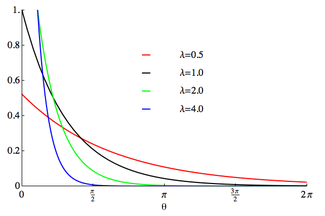
The probability density function of the wrapped exponential distribution is[1]

for where is the rate parameter of the unwrapped distribution. This is identical to the truncated distribution obtained by restricting observed values X from the exponential distribution with rate parameter λ to the range . Note that this distribution is not periodic.

Characteristic function
The characteristic function of the wrapped exponential is just the characteristic function of the exponential function evaluated at integer arguments:

which yields an alternate expression for the wrapped exponential PDF in terms of the circular variable z=e i (θ-m) valid for all real θ and m:
![{\displaystyle {\begin{aligned}f_{WE}(z;\lambda )&={\frac {1}{2\pi }}\sum _{n=-\infty }^{\infty }{\frac {z^{-n}}{1-in/\lambda }}\\[10pt]&={\begin{cases}{\frac {\lambda }{\pi }}\,{\textrm {Im}}(\Phi (z,1,-i\lambda ))-{\frac {1}{2\pi }}&{\text{if }}z\neq 1\\[12pt]{\frac {\lambda }{1-e^{-2\pi \lambda }}}&{\text{if }}z=1\end{cases}}\end{aligned}}}](https://wikimedia.org/api/rest_v1/media/math/render/svg/95e9059afd3d0d8d75dd6cb3cbe6e0acf8cb11b5)
where is the Lerch transcendent function.

Circular moments
In terms of the circular variable the circular moments of the wrapped exponential distribution are the characteristic function of the exponential distribution evaluated at integer arguments:


where is some interval of length . The first moment is then the average value of z, also known as the mean resultant, or mean resultant vector:


The mean angle is

and the length of the mean resultant is

and the variance is then 1-R.
Characterisation
The wrapped exponential distribution is the maximum entropy probability distribution for distributions restricted to the range for a fixed value of the expectation .[1]

See also
References
- ^ a b Jammalamadaka, S. Rao; Kozubowski, Tomasz J. (2004). "New Families of Wrapped Distributions for Modeling Skew Circular Data" (PDF). Communications in Statistics - Theory and Methods. 33 (9): 2059–2074. doi:10.1081/STA-200026570. Retrieved 2011-06-13.