Covariance

Covariance in probability theory and statistics is a measure of the joint variability of two random variables.^[1]

Definition

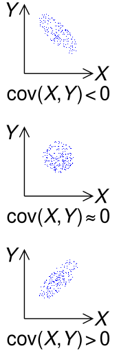
If greater values of one variable mainly correspond with greater values of the other variable, and the same holds for lesser values (that is, the variables tend to show similar behavior), the covariance is positive.^[2] In the opposite case, when greater values of one variable mainly correspond to lesser values of the other (that is, the variables tend to show opposite behavior), the covariance is negative. The sign of the covariance, therefore, shows the tendency in the linear relationship between the variables. The magnitude of the covariance is the geometric mean of the variances that are in common for the two random variables. The correlation coefficient normalizes the covariance by dividing by the geometric mean of the total variances for the two random variables.

A distinction must be made between (1) the covariance of two random variables, which is a population parameter that can be seen as a property of the joint probability distribution, and (2) the sample covariance, which in addition to serving as a descriptor of the sample, also serves as an estimated value of the population parameter.

Mathematics

For two jointly distributed real-valued random variables ${\displaystyle X}$ and ${\displaystyle Y}$ with finite second moments, the covariance is defined as the expected value (or mean) of the product of their deviations from their individual expected values:^{[3][4]: 119}

where ${\displaystyle \operatorname {E} [X]}$ is the expected value of ${\displaystyle X}$, also known as the mean of ${\displaystyle X}$. The covariance is also sometimes denoted ${\displaystyle \sigma _{XY}}$ or ${\displaystyle \sigma (X,Y)}$, in analogy to variance. By using the linearity property of expectations, this can be simplified to the expected value of their product minus the product of their expected values:

but this equation is susceptible to catastrophic cancellation (see the section on numerical computation below).

The units of measurement of the covariance ${\displaystyle \operatorname {cov} (X,Y)}$ are those of ${\displaystyle X}$ times those of ${\displaystyle Y}$. By contrast, correlation coefficients, which depend on the covariance, are a dimensionless measure of linear dependence. (In fact, correlation coefficients can simply be understood as a normalized version of covariance.)

Complex random variables

The covariance between two complex random variables ${\displaystyle Z,W}$ is defined as^[4]: 119

Notice the complex conjugation of the second factor in the definition.

A related pseudo-covariance can also be defined.

Discrete random variables

If the (real) random variable pair ${\displaystyle (X,Y)}$ can take on the values ${\displaystyle (x_{i},y_{i})}$ for ${\displaystyle i=1,\ldots ,n}$, with equal probabilities ${\displaystyle p_{i}=1/n}$, then the covariance can be equivalently written in terms of the means ${\displaystyle \operatorname {E} [X]}$ and ${\displaystyle \operatorname {E} [Y]}$ as

It can also be equivalently expressed, without directly referring to the means, as^[5]

More generally, if there are ${\displaystyle n}$ possible realizations of ${\displaystyle (X,Y)}$, namely ${\displaystyle (x_{i},y_{i})}$ but with possibly unequal probabilities ${\displaystyle p_{i}}$ for ${\displaystyle i=1,\ldots ,n}$, then the covariance is

In the case where two discrete random variables ${\displaystyle X}$ and ${\displaystyle Y}$ have a joint probability distribution, represented by elements ${\displaystyle p_{i,j}}$ corresponding to the joint probabilities of ${\displaystyle P(X=x_{i},Y=y_{j})}$, the covariance is calculated using a double summation over the indices of the matrix:

Examples

Consider 3 independent random variables ${\displaystyle A,B,C}$ and two constants ${\displaystyle q,r}$.

In the special case, ${\displaystyle q=1}$ and ${\displaystyle r=1}$, the covariance between ${\displaystyle X}$ and ${\displaystyle Y}$, is just the variance of ${\displaystyle A}$ and the name covariance is entirely appropriate.

Suppose that ${\displaystyle X}$ and ${\displaystyle Y}$ have the following joint probability mass function,^[6] in which the six central cells give the discrete joint probabilities ${\displaystyle f(x,y)}$ of the six hypothetical realizations ${\displaystyle (x,y)\in S=\left\{(5,8),(6,8),(7,8),(5,9),(6,9),(7,9)\right\}}$:

${\displaystyle f(x,y)}$		x				${\displaystyle f_{Y}(y)}$
		5	6	7
y	8	0	0.4	0.1		0.5
	9	0.3	0	0.2		0.5
${\displaystyle f_{X}(x)}$		0.3	0.4	0.3	1

${\displaystyle X}$ can take on three values (5, 6 and 7) while ${\displaystyle Y}$ can take on two (8 and 9). Their means are ${\displaystyle \mu _{X}=5(0.3)+6(0.4)+7(0.1+0.2)=6}$ and ${\displaystyle \mu _{Y}=8(0.4+0.1)+9(0.3+0.2)=8.5}$. Then,

Properties

Covariance with itself

The variance is a special case of the covariance in which the two variables are identical (that is, in which one variable has the same distribution as the other):^[4]: 121

Covariance of linear combinations

If ${\displaystyle X}$, ${\displaystyle Y}$, ${\displaystyle W}$, and ${\displaystyle V}$ are real-valued random variables and ${\displaystyle a,b,c,d}$ are real-valued constants, then the following facts are a consequence of the definition of covariance:

For a sequence ${\displaystyle X_{1},\ldots ,X_{n}}$ of random variables in real-valued, and constants ${\displaystyle a_{1},\ldots ,a_{n}}$, we have

Hoeffding's covariance identity

A useful identity to compute the covariance between two random variables ${\displaystyle X,Y}$ is the Hoeffding's covariance identity:^[7]

where ${\displaystyle F_{(X,Y)}(x,y)}$ is the joint cumulative distribution function of the random vector ${\displaystyle (X,Y)}$ and ${\displaystyle F_{X}(x),F_{Y}(y)}$ are the marginals.

Uncorrelatedness and independence

Random variables whose covariance is zero are called uncorrelated.^[4]: 121 Similarly, the components of random vectors whose covariance matrix is zero in every entry outside the main diagonal are also called uncorrelated.

If ${\displaystyle X}$ and ${\displaystyle Y}$ are independent random variables, then their covariance is zero.^{[4]: 123 [8]} This follows because under independence,

The converse, however, is not generally true. For example, let ${\displaystyle X}$ be uniformly distributed in ${\displaystyle [-1,1]}$ and let ${\displaystyle Y=X^{2}}$. Clearly, ${\displaystyle X}$ and ${\displaystyle Y}$ are not independent, but

In this case, the relationship between ${\displaystyle Y}$ and ${\displaystyle X}$ is non-linear, while correlation and covariance are measures of linear dependence between two random variables. This example shows that if two random variables are uncorrelated, that does not in general imply that they are independent. However, if two variables are jointly normally distributed (but not if they are merely individually normally distributed), uncorrelatedness does imply independence.^[9]

${\displaystyle X}$ and ${\displaystyle Y}$ whose covariance is positive are called positively correlated, which implies if ${\displaystyle X>E[X]}$ then likely ${\displaystyle Y>E[Y]}$. Conversely, ${\displaystyle X}$ and ${\displaystyle Y}$ with negative covariance are negatively correlated, and if ${\displaystyle X>E[X]}$ then likely ${\displaystyle Y<E[Y]}$.

Relationship to inner products

Many of the properties of covariance can be extracted elegantly by observing that it satisfies similar properties to those of an inner product:

1. bilinear: for constants ${\displaystyle a}$ and ${\displaystyle b}$ and random variables ${\displaystyle X,Y,Z,}$ ${\displaystyle \operatorname {cov} (aX+bY,Z)=a\operatorname {cov} (X,Z)+b\operatorname {cov} (Y,Z)}$
2. symmetric: ${\displaystyle \operatorname {cov} (X,Y)=\operatorname {cov} (Y,X)}$
3. positive semi-definite: ${\displaystyle \sigma ^{2}(X)=\operatorname {cov} (X,X)\geq 0}$ for all random variables ${\displaystyle X}$, and ${\displaystyle \operatorname {cov} (X,X)=0}$ implies that ${\displaystyle X}$ is constant almost surely.

In fact these properties imply that the covariance defines an inner product over the quotient vector space obtained by taking the subspace of random variables with finite second moment and identifying any two that differ by a constant. (This identification turns the positive semi-definiteness above into positive definiteness.) That quotient vector space is isomorphic to the subspace of random variables with finite second moment and mean zero; on that subspace, the covariance is exactly the L² inner product of real-valued functions on the sample space.

As a result, for random variables with finite variance, the inequality

holds via the Cauchy–Schwarz inequality.

Proof: If ${\displaystyle \sigma ^{2}(Y)=0}$, then it holds trivially. Otherwise, let random variable

Then we have

Calculating the sample covariance

The sample covariances among ${\displaystyle K}$ variables based on ${\displaystyle N}$ observations of each, drawn from an otherwise unobserved population, are given by the ${\displaystyle K\times K}$ matrix ${\displaystyle \textstyle {\overline {\mathbf {q} }}=\left[q_{jk}\right]}$ with the entries

${\displaystyle q_{jk}={\frac {1}{N-1}}\sum _{i=1}^{N}\left(X_{ij}-{\bar {X}}_{j}\right)\left(X_{ik}-{\bar {X}}_{k}\right),}$

which is an estimate of the covariance between variable ${\displaystyle j}$ and variable ${\displaystyle k}$.

The sample mean and the sample covariance matrix are unbiased estimates of the mean and the covariance matrix of the random vector ${\displaystyle \textstyle \mathbf {X} }$, a vector whose jth element ${\displaystyle (j=1,\,\ldots ,\,K)}$ is one of the random variables. The reason the sample covariance matrix has ${\displaystyle \textstyle N-1}$ in the denominator rather than ${\displaystyle \textstyle N}$ is essentially that the population mean ${\displaystyle \operatorname {E} (\mathbf {X} )}$ is not known and is replaced by the sample mean ${\displaystyle \mathbf {\bar {X}} }$. If the population mean ${\displaystyle \operatorname {E} (\mathbf {X} )}$ is known, the analogous unbiased estimate is given by

${\displaystyle q_{jk}={\frac {1}{N}}\sum _{i=1}^{N}\left(X_{ij}-\operatorname {E} \left(X_{j}\right)\right)\left(X_{ik}-\operatorname {E} \left(X_{k}\right)\right)}$.

Generalizations

Auto-covariance matrix of real random vectors

For a vector ${\displaystyle \mathbf {X} ={\begin{bmatrix}X_{1}&X_{2}&\dots &X_{m}\end{bmatrix}}^{\mathrm {T} }}$ of ${\displaystyle m}$ jointly distributed random variables with finite second moments, its auto-covariance matrix (also known as the variance–covariance matrix or simply the covariance matrix) ${\displaystyle \operatorname {K} _{\mathbf {X} \mathbf {X} }}$ (also denoted by ${\displaystyle \Sigma (\mathbf {X} )}$ or ${\displaystyle \operatorname {cov} (\mathbf {X} ,\mathbf {X} )}$) is defined as^[10]: 335

Let ${\displaystyle \mathbf {X} }$ be a random vector with covariance matrix Σ, and let A be a matrix that can act on ${\displaystyle \mathbf {X} }$ on the left. The covariance matrix of the matrix-vector product A X is:

This is a direct result of the linearity of expectation and is useful when applying a linear transformation, such as a whitening transformation, to a vector.

Cross-covariance matrix of real random vectors

For real random vectors ${\displaystyle \mathbf {X} \in \mathbb {R} ^{m}}$ and ${\displaystyle \mathbf {Y} \in \mathbb {R} ^{n}}$, the ${\displaystyle m\times n}$ cross-covariance matrix is equal to^[10]: 336

where ${\displaystyle \mathbf {Y} ^{\mathrm {T} }}$ is the transpose of the vector (or matrix) ${\displaystyle \mathbf {Y} }$.

The ${\displaystyle (i,j)}$-th element of this matrix is equal to the covariance ${\displaystyle \operatorname {cov} (X_{i},Y_{j})}$ between the i-th scalar component of ${\displaystyle \mathbf {X} }$ and the j-th scalar component of ${\displaystyle \mathbf {Y} }$. In particular, ${\displaystyle \operatorname {cov} (\mathbf {Y} ,\mathbf {X} )}$ is the transpose of ${\displaystyle \operatorname {cov} (\mathbf {X} ,\mathbf {Y} )}$.

Cross-covariance sesquilinear form of random vectors in a real or complex Hilbert space

More generally let ${\displaystyle H_{1}=(H_{1},\langle \,,\rangle _{1})}$ and ${\displaystyle H_{2}=(H_{2},\langle \,,\rangle _{2})}$, be Hilbert spaces over ${\displaystyle \mathbb {R} }$ or ${\displaystyle \mathbb {C} }$ with ${\displaystyle \langle \,,\rangle }$ anti linear in the first variable, and let ${\displaystyle \mathbf {X} ,\mathbf {Y} }$ be ${\displaystyle H_{1}}$ resp. ${\displaystyle H_{2}}$ valued random variables. Then the covariance of ${\displaystyle \mathbf {X} }$ and ${\displaystyle \mathbf {Y} }$ is the sesquilinear form on ${\displaystyle H_{1}\times H_{2}}$ (anti linear in the first variable) given by

Numerical computation

When ${\displaystyle \operatorname {E} [XY]\approx \operatorname {E} [X]\operatorname {E} [Y]}$, the equation ${\displaystyle \operatorname {cov} (X,Y)=\operatorname {E} \left[XY\right]-\operatorname {E} \left[X\right]\operatorname {E} \left[Y\right]}$ is prone to catastrophic cancellation if ${\displaystyle \operatorname {E} \left[XY\right]}$ and ${\displaystyle \operatorname {E} \left[X\right]\operatorname {E} \left[Y\right]}$ are not computed exactly and thus should be avoided in computer programs when the data has not been centered before.^[11] Numerically stable algorithms should be preferred in this case.^[12]

Comments

The covariance is sometimes called a measure of "linear dependence" between the two random variables. That does not mean the same thing as in the context of linear algebra (see linear dependence). When the covariance is normalized, one obtains the Pearson correlation coefficient, which gives the goodness of the fit for the best possible linear function describing the relation between the variables. In this sense covariance is a linear gauge of dependence.

Applications

In genetics and molecular biology

Covariance is an important measure in biology. Certain sequences of DNA are conserved more than others among species, and thus to study secondary and tertiary structures of proteins, or of RNA structures, sequences are compared in closely related species. If sequence changes are found or no changes at all are found in noncoding RNA (such as microRNA), sequences are found to be necessary for common structural motifs, such as an RNA loop. In genetics, covariance serves a basis for computation of Genetic Relationship Matrix (GRM) (aka kinship matrix), enabling inference on population structure from sample with no known close relatives as well as inference on estimation of heritability of complex traits.

In the theory of evolution and natural selection, the price equation describes how a genetic trait changes in frequency over time. The equation uses a covariance between a trait and fitness, to give a mathematical description of evolution and natural selection. It provides a way to understand the effects that gene transmission and natural selection have on the proportion of genes within each new generation of a population.^[13][14]

In financial economics

Covariances play a key role in financial economics, especially in modern portfolio theory and in the capital asset pricing model. Covariances among various assets' returns are used to determine, under certain assumptions, the relative amounts of different assets that investors should (in a normative analysis) or are predicted to (in a positive analysis) choose to hold in a context of diversification.

In meteorological and oceanographic data assimilation

The covariance matrix is important in estimating the initial conditions required for running weather forecast models, a procedure known as data assimilation. The 'forecast error covariance matrix' is typically constructed between perturbations around a mean state (either a climatological or ensemble mean). The 'observation error covariance matrix' is constructed to represent the magnitude of combined observational errors (on the diagonal) and the correlated errors between measurements (off the diagonal). This is an example of its widespread application to Kalman filtering and more general state estimation for time-varying systems.

In micrometeorology

The eddy covariance technique is a key atmospherics measurement technique where the covariance between instantaneous deviation in vertical wind speed from the mean value and instantaneous deviation in gas concentration is the basis for calculating the vertical turbulent fluxes.

In signal processing

The covariance matrix is used to capture the spectral variability of a signal.^[15]

In statistics and image processing

The covariance matrix is used in principal component analysis to reduce feature dimensionality in data preprocessing.

See also

References

- ^ Rice, John (2007). Mathematical Statistics and Data Analysis. Brooks/Cole Cengage Learning. p. 138. ISBN 9780534399429.
- ^ Weisstein, Eric W. "Covariance". MathWorld.
- ^ Oxford Dictionary of Statistics, Oxford University Press, 2002, p. 104.
- ^ a b c d e Park, Kun Il (2018). Fundamentals of Probability and Stochastic Processes with Applications to Communications. Springer. ISBN 9783319680743.
- ^ Yuli Zhang; Huaiyu Wu; Lei Cheng (June 2012). "Some new deformation formulas about variance and covariance". Proceedings of 4th International Conference on Modelling, Identification and Control(ICMIC2012). pp. 987–992.
- ^ "Covariance of X and Y | STAT 414/415". The Pennsylvania State University. Archived from the original on August 17, 2017. Retrieved August 4, 2019.
- ^ Papoulis (1991). Probability, Random Variables and Stochastic Processes. McGraw-Hill.
- ^ Siegrist, Kyle. "Covariance and Correlation". University of Alabama in Huntsville. Retrieved Oct 3, 2022.
- ^ Dekking, Michel, ed. (2005). A modern introduction to probability and statistics: understandig why and how. Springer texts in statistics. London [Heidelberg]: Springer. ISBN 978-1-85233-896-1.
- ^ a b Gubner, John A. (2006). Probability and Random Processes for Electrical and Computer Engineers. Cambridge University Press. ISBN 978-0-521-86470-1.
- ^ Donald E. Knuth (1998). The Art of Computer Programming, volume 2: Seminumerical Algorithms, 3rd edn., p. 232. Boston: Addison-Wesley.
- ^ Schubert, Erich; Gertz, Michael (2018). "Numerically stable parallel computation of (Co-)variance". Proceedings of the 30th International Conference on Scientific and Statistical Database Management. Bozen-Bolzano, Italy: ACM Press. pp. 1–12. doi:10.1145/3221269.3223036. ISBN 978-1-4503-6505-5. S2CID 49665540.
- ^ Price, George (1970). "Selection and covariance". Nature (journal). 227 (5257): 520–521. Bibcode:1970Natur.227..520P. doi:10.1038/227520a0. PMID 5428476. S2CID 4264723.
- ^ Harman, Oren (2020). "When science mirrors life: on the origins of the Price equation". Philosophical Transactions of the Royal Society B: Biological Sciences. 375 (1797). royalsocietypublishing.org: 1–7. doi:10.1098/rstb.2019.0352. PMC 7133509. PMID 32146891.
- ^ Sahidullah, Md.; Kinnunen, Tomi (March 2016). "Local spectral variability features for speaker verification". Digital Signal Processing. 50: 1–11. doi:10.1016/j.dsp.2015.10.011.