
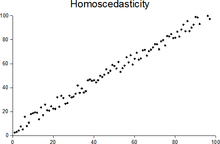
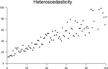
In statistics, a sequence of random variables is homoscedastic (/ˌhoʊmoʊskəˈdæstɪk/) if all its random variables have the same finite variance; this is also known as homogeneity of variance. The complementary notion is called heteroscedasticity, also known as heterogeneity of variance. The spellings homoskedasticity and heteroskedasticity are also frequently used.[1][2][3] Assuming a variable is homoscedastic when in reality it is heteroscedastic (/ˌhɛtəroʊskəˈdæstɪk/) results in unbiased but inefficient point estimates and in biased estimates of standard errors, and may result in overestimating the goodness of fit as measured by the Pearson coefficient.
The existence of heteroscedasticity is a major concern in regression analysis and the analysis of variance, as it invalidates statistical tests of significance that assume that the modelling errors all have the same variance. While the ordinary least squares estimator is still unbiased in the presence of heteroscedasticity, it is inefficient and inference based on the assumption of homoskedasticity is misleading. In that case, generalized least squares (GLS) was frequently used in the past.[4][5] Nowadays, standard practice in econometrics is to include Heteroskedasticity-consistent standard errors instead of using GLS, as GLS can exhibit strong bias in small samples if the actual Skedastic function is unknown.[6]
Because heteroscedasticity concerns expectations of the second moment of the errors, its presence is referred to as misspecification of the second order.[7]
The econometrician Robert Engle was awarded the 2003 Nobel Memorial Prize for Economics for his studies on regression analysis in the presence of heteroscedasticity, which led to his formulation of the autoregressive conditional heteroscedasticity (ARCH) modeling technique.[8]
YouTube Encyclopedic
-
1/5Views:10 03412 9402 500122 73329 436
-
What is Homoskadesticity? (& heteroskedasticity)
-
Homoscedasticity vs Heteroscedasticity | Statistics
-
3.18 - Homoscedasticity vs. Heteroscedasticity in OLS
-
What is Heteroskedasticity?
-
Heteroscedasticity - Introduction
Transcription
Definition
Consider the linear regression equation where the dependent random variable equals the deterministic variable times coefficient plus a random disturbance term that has mean zero. The disturbances are homoscedastic if the variance of is a constant ; otherwise, they are heteroscedastic. In particular, the disturbances are heteroscedastic if the variance of depends on or on the value of . One way they might be heteroscedastic is if (an example of a scedastic function), so the variance is proportional to the value of .


More generally, if the variance-covariance matrix of disturbance across has a nonconstant diagonal, the disturbance is heteroscedastic.[9] The matrices below are covariances when there are just three observations across time. The disturbance in matrix A is homoscedastic; this is the simple case where OLS is the best linear unbiased estimator. The disturbances in matrices B and C are heteroscedastic. In matrix B, the variance is time-varying, increasing steadily across time; in matrix C, the variance depends on the value of . The disturbance in matrix D is homoscedastic because the diagonal variances are constant, even though the off-diagonal covariances are non-zero and ordinary least squares is inefficient for a different reason: serial correlation.

Examples
Heteroscedasticity often occurs when there is a large difference among the sizes of the observations.
A classic example of heteroscedasticity is that of income versus expenditure on meals. A wealthy person may eat inexpensive food sometimes and expensive food at other times. A poor person will almost always eat inexpensive food. Therefore, people with higher incomes exhibit greater variability in expenditures on food.
At a rocket launch, an observer measures the distance traveled by the rocket once per second. In the first couple of seconds, the measurements may be accurate to the nearest centimeter. After five minutes, the accuracy of the measurements may be good only to 100 m, because of the increased distance, atmospheric distortion, and a variety of other factors. So the measurements of distance may exhibit heteroscedasticity.
Consequences
One of the assumptions of the classical linear regression model is that there is no heteroscedasticity. Breaking this assumption means that the Gauss–Markov theorem does not apply, meaning that OLS estimators are not the Best Linear Unbiased Estimators (BLUE) and their variance is not the lowest of all other unbiased estimators. Heteroscedasticity does not cause ordinary least squares coefficient estimates to be biased, although it can cause ordinary least squares estimates of the variance (and, thus, standard errors) of the coefficients to be biased, possibly above or below the true of population variance. Thus, regression analysis using heteroscedastic data will still provide an unbiased estimate for the relationship between the predictor variable and the outcome, but standard errors and therefore inferences obtained from data analysis are suspect. Biased standard errors lead to biased inference, so results of hypothesis tests are possibly wrong. For example, if OLS is performed on a heteroscedastic data set, yielding biased standard error estimation, a researcher might fail to reject a null hypothesis at a given significance level, when that null hypothesis was actually uncharacteristic of the actual population (making a type II error).
Under certain assumptions, the OLS estimator has a normal asymptotic distribution when properly normalized and centered (even when the data does not come from a normal distribution). This result is used to justify using a normal distribution, or a chi square distribution (depending on how the test statistic is calculated), when conducting a hypothesis test. This holds even under heteroscedasticity. More precisely, the OLS estimator in the presence of heteroscedasticity is asymptotically normal, when properly normalized and centered, with a variance-covariance matrix that differs from the case of homoscedasticity. In 1980, White proposed a consistent estimator for the variance-covariance matrix of the asymptotic distribution of the OLS estimator.[2] This validates the use of hypothesis testing using OLS estimators and White's variance-covariance estimator under heteroscedasticity.
Heteroscedasticity is also a major practical issue encountered in ANOVA problems.[10] The F test can still be used in some circumstances.[11]
However, it has been said that students in econometrics should not overreact to heteroscedasticity.[3] One author wrote, "unequal error variance is worth correcting only when the problem is severe."[12] In addition, another word of caution was in the form, "heteroscedasticity has never been a reason to throw out an otherwise good model."[3][13] With the advent of heteroscedasticity-consistent standard errors allowing for inference without specifying the conditional second moment of error term, testing conditional homoscedasticity is not as important as in the past.[6]
For any non-linear model (for instance Logit and Probit models), however, heteroscedasticity has more severe consequences: the maximum likelihood estimates (MLE) of the parameters will usually be biased, as well as inconsistent (unless the likelihood function is modified to correctly take into account the precise form of heteroscedasticity or the distribution is a member of the linear exponential family and the conditional expectation function is correctly specified).[14][15] Yet, in the context of binary choice models (Logit or Probit), heteroscedasticity will only result in a positive scaling effect on the asymptotic mean of the misspecified MLE (i.e. the model that ignores heteroscedasticity).[16] As a result, the predictions which are based on the misspecified MLE will remain correct. In addition, the misspecified Probit and Logit MLE will be asymptotically normally distributed which allows performing the usual significance tests (with the appropriate variance-covariance matrix). However, regarding the general hypothesis testing, as pointed out by Greene, "simply computing a robust covariance matrix for an otherwise inconsistent estimator does not give it redemption. Consequently, the virtue of a robust covariance matrix in this setting is unclear."[17]
Correction
There are several common corrections for heteroscedasticity. They are:
- A stabilizing transformation of the data, e.g. logarithmized data. Non-logarithmized series that are growing exponentially often appear to have increasing variability as the series rises over time. The variability in percentage terms may, however, be rather stable.
- Use a different specification for the model (different X variables, or perhaps non-linear transformations of the X variables).
- Apply a weighted least squares estimation method, in which OLS is applied to transformed or weighted values of X and Y. The weights vary over observations, usually depending on the changing error variances. In one variation the weights are directly related to the magnitude of the dependent variable, and this corresponds to least squares percentage regression.[18]
- Heteroscedasticity-consistent standard errors (HCSE), while still biased, improve upon OLS estimates.[2] HCSE is a consistent estimator of standard errors in regression models with heteroscedasticity. This method corrects for heteroscedasticity without altering the values of the coefficients. This method may be superior to regular OLS because if heteroscedasticity is present it corrects for it, however, if the data is homoscedastic, the standard errors are equivalent to conventional standard errors estimated by OLS. Several modifications of the White method of computing heteroscedasticity-consistent standard errors have been proposed as corrections with superior finite sample properties.
- Wild bootstrapping can be used as a Resampling method that respects the differences in the conditional variance of the error term. An alternative is resampling observations instead of errors. Note resampling errors without respect for the affiliated values of the observation enforces homoskedasticity and thus yields incorrect inference.
- Use MINQUE or even the customary estimators (for independent samples with observations each), whose efficiency losses are not substantial when the number of observations per sample is large (), especially for small number of independent samples.[19]


Testing

Residuals can be tested for homoscedasticity using the Breusch–Pagan test,[20] which performs an auxiliary regression of the squared residuals on the independent variables. From this auxiliary regression, the explained sum of squares is retained, divided by two, and then becomes the test statistic for a chi-squared distribution with the degrees of freedom equal to the number of independent variables.[21] The null hypothesis of this chi-squared test is homoscedasticity, and the alternative hypothesis would indicate heteroscedasticity. Since the Breusch–Pagan test is sensitive to departures from normality or small sample sizes, the Koenker–Bassett or 'generalized Breusch–Pagan' test is commonly used instead.[22][additional citation(s) needed] From the auxiliary regression, it retains the R-squared value which is then multiplied by the sample size, and then becomes the test statistic for a chi-squared distribution (and uses the same degrees of freedom). Although it is not necessary for the Koenker–Bassett test, the Breusch–Pagan test requires that the squared residuals also be divided by the residual sum of squares divided by the sample size.[22] Testing for groupwise heteroscedasticity can be done with the Goldfeld–Quandt test.[23]
Due to the standard use of heteroskedasticity-consistent Standard Errors and the problem of Pre-test, econometricians nowadays rarely use tests for conditional heteroskedasticity.[6]
List of tests
Although tests for heteroscedasticity between groups can formally be considered as a special case of testing within regression models, some tests have structures specific to this case.
- Tests in regression
- Tests for grouped data
Generalisations
Homoscedastic distributions
Two or more normal distributions, are both homoscedastic and lack Serial correlation if they share the same diagonals in their covariance matrix, and their non-diagonal entries are zero. Homoscedastic distributions are especially useful to derive statistical pattern recognition and machine learning algorithms. One popular example of an algorithm that assumes homoscedasticity is Fisher's linear discriminant analysis. The concept of homoscedasticity can be applied to distributions on spheres.[27]


Multivariate data
The study of homescedasticity and heteroscedasticity has been generalized to the multivariate case, which deals with the covariances of vector observations instead of the variance of scalar observations. One version of this is to use covariance matrices as the multivariate measure of dispersion. Several authors have considered tests in this context, for both regression and grouped-data situations.[28][29] Bartlett's test for heteroscedasticity between grouped data, used most commonly in the univariate case, has also been extended for the multivariate case, but a tractable solution only exists for 2 groups.[30] Approximations exist for more than two groups, and they are both called Box's M test.
See also
References
- ^ For the Greek etymology of the term, see McCulloch, J. Huston (1985). "On Heteros*edasticity". Econometrica. 53 (2): 483. JSTOR 1911250.
- ^ a b c d White, Halbert (1980). "A heteroskedasticity-consistent covariance matrix estimator and a direct test for heteroskedasticity". Econometrica. 48 (4): 817–838. CiteSeerX 10.1.1.11.7646. doi:10.2307/1912934. JSTOR 1912934.
- ^ a b c Gujarati, D. N.; Porter, D. C. (2009). Basic Econometrics (Fifth ed.). Boston: McGraw-Hill Irwin. p. 400. ISBN 9780073375779.
- ^ Goldberger, Arthur S. (1964). Econometric Theory. New York: John Wiley & Sons. pp. 238–243. ISBN 9780471311010.
- ^ Johnston, J. (1972). Econometric Methods. New York: McGraw-Hill. pp. 214–221.
- ^ a b c Angrist, Joshua D.; Pischke, Jörn-Steffen (2009-12-31). Mostly Harmless Econometrics: An Empiricist's Companion. Princeton University Press. doi:10.1515/9781400829828. ISBN 978-1-4008-2982-8.
- ^ Long, J. Scott; Trivedi, Pravin K. (1993). "Some Specification Tests for the Linear Regression Model". In Bollen, Kenneth A.; Long, J. Scott (eds.). Testing Structural Equation Models. London: Sage. pp. 66–110. ISBN 978-0-8039-4506-7.
- ^ Engle, Robert F. (July 1982). "Autoregressive Conditional Heteroscedasticity with Estimates of the Variance of United Kingdom Inflation". Econometrica. 50 (4): 987–1007. doi:10.2307/1912773. ISSN 0012-9682. JSTOR 1912773.
- ^ Peter Kennedy, A Guide to Econometrics, 5th edition, p. 137.
- ^ Jinadasa, Gamage; Weerahandi, Sam (1998). "Size performance of some tests in one-way anova". Communications in Statistics - Simulation and Computation. 27 (3): 625. doi:10.1080/03610919808813500.
- ^ Bathke, A (2004). "The ANOVA F test can still be used in some balanced designs with unequal variances and nonnormal data". Journal of Statistical Planning and Inference. 126 (2): 413–422. doi:10.1016/j.jspi.2003.09.010.
- ^ Fox, J. (1997). Applied Regression Analysis, Linear Models, and Related Methods. California: Sage Publications. p. 306. (Cited in Gujarati et al. 2009, p. 400)
- ^ Mankiw, N. G. (1990). "A Quick Refresher Course in Macroeconomics". Journal of Economic Literature. 28 (4): 1645–1660 [p. 1648]. doi:10.3386/w3256. JSTOR 2727441.
- ^ Giles, Dave (May 8, 2013). "Robust Standard Errors for Nonlinear Models". Econometrics Beat.
- ^ Gourieroux, C.; Monfort, A.; Trognon, A. (1984). "Pseudo Maximum Likelihood Methods: Theory". Econometrica. 52 (3): 681–700. doi:10.2307/1913471. ISSN 0012-9682.
- ^ Ginker, T.; Lieberman, O. (2017). "Robustness of binary choice models to conditional heteroscedasticity". Economics Letters. 150: 130–134. doi:10.1016/j.econlet.2016.11.024.
- ^ Greene, William H. (2012). "Estimation and Inference in Binary Choice Models". Econometric Analysis (Seventh ed.). Boston: Pearson Education. pp. 730–755 [p. 733]. ISBN 978-0-273-75356-8.
- ^ Tofallis, C (2008). "Least Squares Percentage Regression". Journal of Modern Applied Statistical Methods. 7: 526–534. doi:10.2139/ssrn.1406472. SSRN 1406472.
- ^ J. N. K. Rao (March 1973). "On the Estimation of Heteroscedastic Variances". Biometrics. 29 (1): 11–24. doi:10.2307/2529672. JSTOR 2529672.
- ^ Breusch, T. S.; Pagan, A. R. (1979). "A Simple Test for Heteroscedasticity and Random Coefficient Variation". Econometrica. 47 (5): 1287–1294. doi:10.2307/1911963. ISSN 0012-9682. JSTOR 1911963.
- ^ Ullah, Muhammad Imdad (2012-07-26). "Breusch Pagan Test for Heteroscedasticity". Basic Statistics and Data Analysis. Retrieved 2020-11-28.
- ^ a b Pryce, Gwilym. "Heteroscedasticity: Testing and Correcting in SPSS" (PDF). pp. 12–18. Archived (PDF) from the original on 2017-03-27. Retrieved 26 March 2017.
- ^ Baum, Christopher F. (2006). "Stata Tip 38: Testing for Groupwise Heteroskedasticity". The Stata Journal: Promoting Communications on Statistics and Stata. 6 (4): 590–592. doi:10.1177/1536867X0600600412. ISSN 1536-867X. S2CID 117349246.
- ^ R. E. Park (1966). "Estimation with Heteroscedastic Error Terms". Econometrica. 34 (4): 888. doi:10.2307/1910108. JSTOR 1910108.
- ^ Glejser, H. (1969). "A new test for heteroscedasticity". Journal of the American Statistical Association. 64 (325): 316–323. doi:10.1080/01621459.1969.10500976.
- ^ Machado, José A. F.; Silva, J. M. C. Santos (2000). "Glejser's test revisited". Journal of Econometrics. 97 (1): 189–202. doi:10.1016/S0304-4076(00)00016-6.
- ^ Hamsici, Onur C.; Martinez, Aleix M. (2007) "Spherical-Homoscedastic Distributions: The Equivalency of Spherical and Normal Distributions in Classification", Journal of Machine Learning Research, 8, 1583-1623
- ^ Holgersson, H. E. T.; Shukur, G. (2004). "Testing for multivariate heteroscedasticity". Journal of Statistical Computation and Simulation. 74 (12): 879. doi:10.1080/00949650410001646979. hdl:2077/24416. S2CID 121576769.
- ^ Gupta, A. K.; Tang, J. (1984). "Distribution of likelihood ratio statistic for testing equality of covariance matrices of multivariate Gaussian models". Biometrika. 71 (3): 555–559. doi:10.1093/biomet/71.3.555. JSTOR 2336564.
- ^ d'Agostino, R. B.; Russell, H. K. (2005). "Multivariate Bartlett Test". Encyclopedia of Biostatistics. doi:10.1002/0470011815.b2a13048. ISBN 978-0470849071.
Further reading
Most statistics textbooks will include at least some material on homoscedasticity and heteroscedasticity. Some examples are:
- Asteriou, Dimitros; Hall, Stephen G. (2011). Applied Econometrics (Second ed.). Palgrave MacMillan. pp. 109–147. ISBN 978-0-230-27182-1.
- Davidson, Russell; MacKinnon, James G. (1993). Estimation and Inference in Econometrics. New York: Oxford University Press. pp. 547–582. ISBN 978-0-19-506011-9.
- Dougherty, Christopher (2011). Introduction to Econometrics. New York: Oxford University Press. pp. 280–299. ISBN 978-0-19-956708-9.
- Gujarati, Damodar N.; Porter, Dawn C. (2009). Basic Econometrics (Fifth ed.). New York: McGraw-Hill Irwin. pp. 365–411. ISBN 978-0-07-337577-9.
- Kmenta, Jan (1986). Elements of Econometrics (Second ed.). New York: Macmillan. pp. 269–298. ISBN 978-0-02-365070-3.
- Maddala, G. S.; Lahiri, Kajal (2009). Introduction to Econometrics (Fourth ed.). New York: Wiley. pp. 211–238. ISBN 978-0-470-01512-4.