Bilinear interpolation

In mathematics, bilinear interpolation is a method for interpolating functions of two variables (e.g., x and y) using repeated linear interpolation. It is usually applied to functions sampled on a 2D rectilinear grid, though it can be generalized to functions defined on the vertices of (a mesh of) arbitrary convex quadrilaterals.

Bilinear interpolation is performed using linear interpolation first in one direction, and then again in another direction. Although each step is linear in the sampled values and in the position, the interpolation as a whole is not linear but rather quadratic in the sample location.

Bilinear interpolation is one of the basic resampling techniques in computer vision and image processing, where it is also called bilinear filtering or bilinear texture mapping.

Computation

Suppose that we want to find the value of the unknown function f at the point (x, y). It is assumed that we know the value of f at the four points Q₁₁ = (x₁, y₁), Q₁₂ = (x₁, y₂), Q₂₁ = (x₂, y₁), and Q₂₂ = (x₂, y₂).

Repeated linear interpolation

We first do linear interpolation in the x-direction. This yields

${\displaystyle {\begin{aligned}f(x,y_{1})={\frac {x_{2}-x}{x_{2}-x_{1}}}f(Q_{11})+{\frac {x-x_{1}}{x_{2}-x_{1}}}f(Q_{21}),\\f(x,y_{2})={\frac {x_{2}-x}{x_{2}-x_{1}}}f(Q_{12})+{\frac {x-x_{1}}{x_{2}-x_{1}}}f(Q_{22}).\end{aligned}}}$

We proceed by interpolating in the y-direction to obtain the desired estimate:

${\displaystyle {\begin{aligned}f(x,y)&={\frac {y_{2}-y}{y_{2}-y_{1}}}f(x,y_{1})+{\frac {y-y_{1}}{y_{2}-y_{1}}}f(x,y_{2})\\&={\frac {y_{2}-y}{y_{2}-y_{1}}}\left({\frac {x_{2}-x}{x_{2}-x_{1}}}f(Q_{11})+{\frac {x-x_{1}}{x_{2}-x_{1}}}f(Q_{21})\right)+{\frac {y-y_{1}}{y_{2}-y_{1}}}\left({\frac {x_{2}-x}{x_{2}-x_{1}}}f(Q_{12})+{\frac {x-x_{1}}{x_{2}-x_{1}}}f(Q_{22})\right)\\&={\frac {1}{(x_{2}-x_{1})(y_{2}-y_{1})}}\left(f(Q_{11})(x_{2}-x)(y_{2}-y)+f(Q_{21})(x-x_{1})(y_{2}-y)+f(Q_{12})(x_{2}-x)(y-y_{1})+f(Q_{22})(x-x_{1})(y-y_{1})\right)\\&={\frac {1}{(x_{2}-x_{1})(y_{2}-y_{1})}}{\begin{bmatrix}x_{2}-x&x-x_{1}\end{bmatrix}}{\begin{bmatrix}f(Q_{11})&f(Q_{12})\\f(Q_{21})&f(Q_{22})\end{bmatrix}}{\begin{bmatrix}y_{2}-y\\y-y_{1}\end{bmatrix}}.\end{aligned}}}$

Note that we will arrive at the same result if the interpolation is done first along the y direction and then along the x direction.^[1]

Polynomial fit

An alternative way is to write the solution to the interpolation problem as a multilinear polynomial

${\displaystyle f(x,y)\approx a_{00}+a_{10}x+a_{01}y+a_{11}xy,}$

where the coefficients are found by solving the linear system

${\displaystyle {\begin{aligned}{\begin{bmatrix}1&x_{1}&y_{1}&x_{1}y_{1}\\1&x_{1}&y_{2}&x_{1}y_{2}\\1&x_{2}&y_{1}&x_{2}y_{1}\\1&x_{2}&y_{2}&x_{2}y_{2}\end{bmatrix}}{\begin{bmatrix}a_{00}\\a_{10}\\a_{01}\\a_{11}\end{bmatrix}}={\begin{bmatrix}f(Q_{11})\\f(Q_{12})\\f(Q_{21})\\f(Q_{22})\end{bmatrix}},\end{aligned}}}$

yielding the result

${\displaystyle {\begin{aligned}{\begin{bmatrix}a_{00}\\a_{10}\\a_{01}\\a_{11}\end{bmatrix}}={\frac {1}{(x_{2}-x_{1})(y_{2}-y_{1})}}{\begin{bmatrix}x_{2}y_{2}&-x_{2}y_{1}&-x_{1}y_{2}&x_{1}y_{1}\\-y_{2}&y_{1}&y_{2}&-y_{1}\\-x_{2}&x_{2}&x_{1}&-x_{1}\\1&-1&-1&1\end{bmatrix}}{\begin{bmatrix}f(Q_{11})\\f(Q_{12})\\f(Q_{21})\\f(Q_{22})\end{bmatrix}}.\end{aligned}}}$

Weighted mean

The solution can also be written as a weighted mean of the f(Q):

${\displaystyle f(x,y)\approx w_{11}f(Q_{11})+w_{12}f(Q_{12})+w_{21}f(Q_{21})+w_{22}f(Q_{22}),}$

where the weights sum to 1 and satisfy the transposed linear system

${\displaystyle {\begin{bmatrix}1&1&1&1\\x_{1}&x_{1}&x_{2}&x_{2}\\y_{1}&y_{2}&y_{1}&y_{2}\\x_{1}y_{1}&x_{1}y_{2}&x_{2}y_{1}&x_{2}y_{2}\end{bmatrix}}{\begin{bmatrix}w_{11}\\w_{12}\\w_{21}\\w_{22}\end{bmatrix}}={\begin{bmatrix}1\\x\\y\\xy\end{bmatrix}},}$

yielding the result

${\displaystyle {\begin{aligned}{\begin{bmatrix}w_{11}\\w_{21}\\w_{12}\\w_{22}\end{bmatrix}}={\frac {1}{(x_{2}-x_{1})(y_{2}-y_{1})}}{\begin{bmatrix}x_{2}y_{2}&-y_{2}&-x_{2}&1\\-x_{2}y_{1}&y_{1}&x_{2}&-1\\-x_{1}y_{2}&y_{2}&x_{1}&-1\\x_{1}y_{1}&-y_{1}&-x_{1}&1\end{bmatrix}}{\begin{bmatrix}1\\x\\y\\xy\end{bmatrix}},\end{aligned}}}$

which simplifies to

${\displaystyle {\begin{aligned}w_{11}&=(x_{2}-x)(y_{2}-y)/((x_{2}-x_{1})(y_{2}-y_{1})),\\w_{12}&=(x_{2}-x)(y-y_{1})/((x_{2}-x_{1})(y_{2}-y_{1})),\\w_{21}&=(x-x_{1})(y_{2}-y)/((x_{2}-x_{1})(y_{2}-y_{1})),\\w_{22}&=(x-x_{1})(y-y_{1})/((x_{2}-x_{1})(y_{2}-y_{1})),\end{aligned}}}$

in agreement with the result obtained by repeated linear interpolation. The set of weights can also be interpreted as a set of generalized barycentric coordinates for a rectangle.

Alternative matrix form

Combining the above, we have

${\displaystyle {\begin{aligned}f(x,y)\approx {\frac {1}{(x_{2}-x_{1})(y_{2}-y_{1})}}{\begin{bmatrix}f(Q_{11})&f(Q_{12})&f(Q_{21})&f(Q_{22})\end{bmatrix}}{\begin{bmatrix}x_{2}y_{2}&-y_{2}&-x_{2}&1\\-x_{2}y_{1}&y_{1}&x_{2}&-1\\-x_{1}y_{2}&y_{2}&x_{1}&-1\\x_{1}y_{1}&-y_{1}&-x_{1}&1\end{bmatrix}}{\begin{bmatrix}1\\x\\y\\xy\end{bmatrix}}.\end{aligned}}}$

On the unit square

If we choose a coordinate system in which the four points where f is known are (0, 0), (0, 1), (1, 0), and (1, 1), then the interpolation formula simplifies to

${\displaystyle f(x,y)\approx f(0,0)(1-x)(1-y)+f(0,1)(1-x)y+f(1,0)x(1-y)+f(1,1)xy,}$

or equivalently, in matrix operations:

${\displaystyle f(x,y)\approx {\begin{bmatrix}1-x&x\end{bmatrix}}{\begin{bmatrix}f(0,0)&f(0,1)\\f(1,0)&f(1,1)\end{bmatrix}}{\begin{bmatrix}1-y\\y\end{bmatrix}}.}$

Here we also recognize the weights:

${\displaystyle {\begin{aligned}w_{11}&=(1-x)(1-y),\\w_{12}&=(1-x)y,\\w_{21}&=x(1-y),\\w_{22}&=xy.\end{aligned}}}$

Alternatively, the interpolant on the unit square can be written as

${\displaystyle f(x,y)=a_{00}+a_{10}x+a_{01}y+a_{11}xy,}$

where

${\displaystyle {\begin{aligned}a_{00}&=f(0,0),\\a_{10}&=f(1,0)-f(0,0),\\a_{01}&=f(0,1)-f(0,0),\\a_{11}&=f(1,1)-f(1,0)-f(0,1)+f(0,0).\end{aligned}}}$

In both cases, the number of constants (four) correspond to the number of data points where f is given.

Properties

As the name suggests, the bilinear interpolant is not linear; but it is linear (i.e. affine) along lines parallel to either the x or the y direction, equivalently if x or y is held constant. Along any other straight line, the interpolant is quadratic. Even though the interpolation is not linear in the position (x and y), at a fixed point it is linear in the interpolation values, as can be seen in the (matrix) equations above.

The result of bilinear interpolation is independent of which axis is interpolated first and which second. If we had first performed the linear interpolation in the y direction and then in the x direction, the resulting approximation would be the same.

The interpolant is a bilinear polynomial, which is also a harmonic function satisfying Laplace's equation. Its graph is a bilinear Bézier surface patch.

Inverse and generalization

In general, the interpolant will assume any value (in the convex hull of the vertex values) at an infinite number of points (forming branches of hyperbolas^[2]), so the interpolation is not invertible.

However, when bilinear interpolation is applied to two functions simultaneously, such as when interpolating a vector field, then the interpolation is invertible (under certain conditions). In particular, this inverse can be used to find the "unit square coordinates" of a point inside any convex quadrilateral (by considering the coordinates of the quadrilateral as a vector field which is bilinearly interpolated on the unit square). Using this procedure bilinear interpolation can be extended to any convex quadrilateral, though the computation is significantly more complicated if it is not a parallelogram.^[3] The resulting map between quadrilaterals is known as a bilinear transformation, bilinear warp or bilinear distortion.

Alternatively, a projective mapping between a quadrilateral and the unit square may be used, but the resulting interpolant will not be bilinear.

In the special case when the quadrilateral is a parallelogram, a linear mapping to the unit square exists and the generalization follows easily.

The obvious extension of bilinear interpolation to three dimensions is called trilinear interpolation.

Inverse computation

Let ${\textstyle F}$ be a vector field that is bilinearly interpolated on the unit square parameterized by ${\textstyle \mu ,\lambda \in [0,1]}$. Inverting the interpolation requires solving a system of two bilinear polynomial equations: $${\displaystyle A+B\lambda +C\mu +D\lambda \mu =0}$$ where $${\displaystyle {\begin{aligned}A&=F_{00}-F\\B&=F_{10}-F_{00}\\C&=F_{01}-F_{00}\\D&=F_{11}-F_{01}-F_{10}+F_{00}\end{aligned}}}$$ Taking a 2-d cross product (see Grassman product) of the system with a carefully chosen vectors allows us to eliminate terms: $${\displaystyle {\begin{aligned}(A+B\lambda +C\mu )&\times D&=0\\(A+B\lambda )&\times (C+D\lambda )&=0\\(A+C\mu )&\times (B+D\mu )&=0\\\end{aligned}}}$$ which expands to $${\displaystyle {\begin{aligned}c+e\lambda +f\mu &=0\\b+(c+d)\lambda +e\lambda ^{2}&=0\\a+(c-d)\mu +f\mu ^{2}&=0\\\end{aligned}}}$$ where $${\displaystyle {\begin{aligned}a&=A\times B\\b&=A\times C\qquad d=B\times C\\c&=A\times D\qquad e=B\times D\qquad f=C\times D\end{aligned}}}$$ The quadratic equations can be solved using the quadratic formula. We have the equivalent determinants $${\displaystyle \mathbb {D} =(c+d)^{2}-4eb=(c-d)^{2}-4fa}$$ and the solutions $${\displaystyle \lambda ={\frac {-c-d\pm {\sqrt {\mathbb {D} }}}{2e}}\qquad \mu ={\frac {-c+d\mp {\sqrt {\mathbb {D} }}}{2f}}}$$ (opposite signs are enforced by the linear relation). The cases when ${\displaystyle e=0}$ or ${\displaystyle f=0}$ must be handled separately. Given the right conditions, one of the two solutions should be in the unit square.

Application in image processing

In computer vision and image processing, bilinear interpolation is used to resample images and textures. An algorithm is used to map a screen pixel location to a corresponding point on the texture map. A weighted average of the attributes (color, transparency, etc.) of the four surrounding texels is computed and applied to the screen pixel. This process is repeated for each pixel forming the object being textured.^[4]

When an image needs to be scaled up, each pixel of the original image needs to be moved in a certain direction based on the scale constant. However, when scaling up an image by a non-integral scale factor, there are pixels (i.e., holes) that are not assigned appropriate pixel values. In this case, those holes should be assigned appropriate RGB or grayscale values so that the output image does not have non-valued pixels.

Bilinear interpolation can be used where perfect image transformation with pixel matching is impossible, so that one can calculate and assign appropriate intensity values to pixels. Unlike other interpolation techniques such as nearest-neighbor interpolation and bicubic interpolation, bilinear interpolation uses values of only the 4 nearest pixels, located in diagonal directions from a given pixel, in order to find the appropriate color intensity values of that pixel.

Bilinear interpolation considers the closest 2 × 2 neighborhood of known pixel values surrounding the unknown pixel's computed location. It then takes a weighted average of these 4 pixels to arrive at its final, interpolated value.^[5][6]

Example

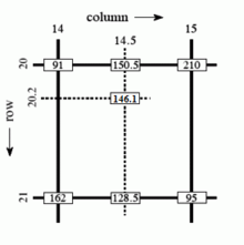
As seen in the example on the right, the intensity value at the pixel computed to be at row 20.2, column 14.5 can be calculated by first linearly interpolating between the values at column 14 and 15 on each rows 20 and 21, giving

${\displaystyle {\begin{aligned}I_{20,14.5}&={\frac {15-14.5}{15-14}}\cdot 91+{\frac {14.5-14}{15-14}}\cdot 210=150.5,\\I_{21,14.5}&={\frac {15-14.5}{15-14}}\cdot 162+{\frac {14.5-14}{15-14}}\cdot 95=128.5,\end{aligned}}}$

and then interpolating linearly between these values, giving

${\displaystyle I_{20.2,14.5}={\frac {21-20.2}{21-20}}\cdot 150.5+{\frac {20.2-20}{21-20}}\cdot 128.5=146.1.}$

This algorithm reduces some of the visual distortion caused by resizing an image to a non-integral zoom factor, as opposed to nearest-neighbor interpolation, which will make some pixels appear larger than others in the resized image.

See also

• Bicubic interpolation
• Trilinear interpolation
• Spline interpolation
• Lanczos resampling
• Stairstep interpolation
• Barycentric coordinates - for interpolating within a triangle or tetrahedron

References

This page was last edited on 17 February 2024, at 08:29

References

- ^ Press, William H.; Teukolsky, Saul A.; Vetterling, William T.; Flannery, Brian P. (1992). Numerical recipes in C: the art of scientific computing (2nd ed.). New York, NY, USA: Cambridge University Press. pp. 123-128. ISBN 0-521-43108-5.
- ^ Monasse, Pascal (2019-08-10). "Extraction of the Level Lines of a Bilinear Image". Image Processing on Line. 9: 205–219. doi:10.5201/ipol.2019.269. ISSN 2105-1232.
- ^ Quilez, Inigo (2010). "Inverse bilinear interpolation". iquilezles.org. Archived from the original on 2010-08-13. Retrieved 2024-02-17.
- ^ Bilinear interpolation definition (popular article on www.pcmag.com.
- ^ Khosravi, M. R. (2021-03-19). "BL-ALM: A Blind Scalable Edge-Guided Reconstruction Filter for Smart Environmental Monitoring Through Green IoMT-UAV Networks". IEEE Transactions on Green Communications and Networking. 5 (2): 727–736. doi:10.1109/TGCN.2021.3067555. S2CID 233669511.
- ^ "Web tutorial: Digital Image Interpolation".