Spectral clustering

In multivariate statistics, spectral clustering techniques make use of the spectrum (eigenvalues) of the similarity matrix of the data to perform dimensionality reduction before clustering in fewer dimensions. The similarity matrix is provided as an input and consists of a quantitative assessment of the relative similarity of each pair of points in the dataset.

In application to image segmentation, spectral clustering is known as segmentation-based object categorization.

Definitions

Given an enumerated set of data points, the similarity matrix may be defined as a symmetric matrix ${\displaystyle A}$, where ${\displaystyle A_{ij}\geq 0}$ represents a measure of the similarity between data points with indices ${\displaystyle i}$ and ${\displaystyle j}$. The general approach to spectral clustering is to use a standard clustering method (there are many such methods, k-means is discussed below) on relevant eigenvectors of a Laplacian matrix of ${\displaystyle A}$. There are many different ways to define a Laplacian which have different mathematical interpretations, and so the clustering will also have different interpretations. The eigenvectors that are relevant are the ones that correspond to several smallest eigenvalues of the Laplacian except for the smallest eigenvalue which will have a value of 0. For computational efficiency, these eigenvectors are often computed as the eigenvectors corresponding to the largest several eigenvalues of a function of the Laplacian.

Laplacian matrix

Spectral clustering is well known to relate to partitioning of a mass-spring system, where each mass is associated with a data point and each spring stiffness corresponds to a weight of an edge describing a similarity of the two related data points, as in the spring system. Specifically, the classical reference ^[1] explains that the eigenvalue problem describing transversal vibration modes of a mass-spring system is exactly the same as the eigenvalue problem for the graph Laplacian matrix defined as

${\displaystyle L:=D-A}$,

where ${\displaystyle D}$ is the diagonal matrix

${\displaystyle D_{ii}=\sum _{j}A_{ij},}$

and A is the adjacency matrix.

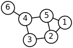
The masses that are tightly connected by the springs in the mass-spring system evidently move together from the equilibrium position in low-frequency vibration modes, so that the components of the eigenvectors corresponding to the smallest eigenvalues of the graph Laplacian can be used for meaningful clustering of the masses. For example, assuming that all the springs and the masses are identical in the 2-dimensional spring system pictured, one would intuitively expect that the loosest connected masses on the right-hand side of the system would move with the largest amplitude and in the opposite direction to the rest of the masses when the system is shaken — and this expectation will be confirmed by analyzing components of the eigenvectors of the graph Laplacian corresponding to the smallest eigenvalues, i.e., the smallest vibration frequencies.

Laplacian matrix normalization

The goal of normalization is making the diagonal entries of the Laplacian matrix to be all unit, also scaling off-diagonal entries correspondingly. In a weighted graph, a vertex may have a large degree because of a small number of connected edges but with large weights just as well as due to a large number of connected edges with unit weights.

A popular normalized spectral clustering technique is the normalized cuts algorithm or Shi–Malik algorithm introduced by Jianbo Shi and Jitendra Malik,^[2] commonly used for image segmentation. It partitions points into two sets ${\displaystyle (B_{1},B_{2})}$ based on the eigenvector ${\displaystyle v}$ corresponding to the second-smallest eigenvalue of the symmetric normalized Laplacian defined as

${\displaystyle L^{\text{norm}}:=I-D^{-1/2}AD^{-1/2}.}$

The vector ${\displaystyle v}$ is also the eigenvector corresponding to the second-largest eigenvalue of the symmetrically normalized adjacency matrix ${\displaystyle D^{-1/2}AD^{-1/2}.}$

The random walk (or left) normalized Laplacian is defined as

${\displaystyle L^{\text{rw}}:=D^{-1}L=I-D^{-1}A}$

and can also be used for spectral clustering. A mathematically equivalent algorithm ^[3] takes the eigenvector ${\displaystyle u}$ corresponding to the largest eigenvalue of the random walk normalized adjacency matrix ${\displaystyle P=D^{-1}A}$.

The eigenvector ${\displaystyle v}$ of the symmetrically normalized Laplacian and the eigenvector ${\displaystyle u}$ of the left normalized Laplacian are related by the identity ${\displaystyle D^{-1/2}v=u.}$

Cluster analysis via Spectral Embedding

Knowing the ${\displaystyle n}$-by-${\displaystyle k}$ matrix ${\displaystyle V}$ of selected eigenvectors, mapping — called spectral embedding — of the original ${\displaystyle n}$ data points is performed to a ${\displaystyle k}$-dimensional vector space using the rows of ${\displaystyle V}$. Now the analysis is reduced to clustering vectors with ${\displaystyle k}$ components, which may be done in various ways.

In the simplest case ${\displaystyle k=1}$, the selected single eigenvector ${\displaystyle v}$, called the Fiedler vector, corresponds to the second smallest eigenvalue. Using the components of ${\displaystyle v,}$ one can place all points whose component in ${\displaystyle v}$ is positive in the set ${\displaystyle B_{+}}$ and the rest in ${\displaystyle B_{-}}$, thus bi-partitioning the graph and labeling the data points with two labels. This sign-based approach follows the intuitive explanation of spectral clustering via the mass-spring model — in the low frequency vibration mode that the Fiedler vector ${\displaystyle v}$ represents, one cluster data points identified with mutually strongly connected masses would move together in one direction, while in the complement cluster data points identified with remaining masses would move together in the opposite direction. The algorithm can be used for hierarchical clustering by repeatedly partitioning the subsets in the same fashion.

In the general case ${\displaystyle k>1}$, any vector clustering technique can be used, e.g., DBSCAN.

Algorithms

Basic Algorithm

1. Calculate the Laplacian ${\displaystyle L}$ (or the normalized Laplacian)
2. Calculate the first ${\displaystyle k}$ eigenvectors (the eigenvectors corresponding to the ${\displaystyle k}$ smallest eigenvalues of ${\displaystyle L}$)
3. Consider the matrix formed by the first ${\displaystyle k}$ eigenvectors; the ${\displaystyle l}$-th row defines the features of graph node ${\displaystyle l}$
4. Cluster the graph nodes based on these features (e.g., using k-means clustering)

If the similarity matrix ${\displaystyle A}$ has not already been explicitly constructed, the efficiency of spectral clustering may be improved if the solution to the corresponding eigenvalue problem is performed in a matrix-free fashion (without explicitly manipulating or even computing the similarity matrix), as in the Lanczos algorithm.

For large-sized graphs, the second eigenvalue of the (normalized) graph Laplacian matrix is often ill-conditioned, leading to slow convergence of iterative eigenvalue solvers. Preconditioning is a key technology accelerating the convergence, e.g., in the matrix-free LOBPCG method. Spectral clustering has been successfully applied on large graphs by first identifying their community structure, and then clustering communities.^[4]

Spectral clustering is closely related to nonlinear dimensionality reduction, and dimension reduction techniques such as locally-linear embedding can be used to reduce errors from noise or outliers.^[5]

Costs

Denoting the number of the data points by ${\displaystyle n}$, it is important to estimate the memory footprint and compute time, or number of arithmetic operations (AO) performed, as a function of ${\displaystyle n}$. No matter the algorithm of the spectral clustering, the two main costly items are the construction of the graph Laplacian and determining its ${\displaystyle k}$ eigenvectors for the spectral embedding. The last step — determining the labels from the ${\displaystyle n}$-by-${\displaystyle k}$ matrix of eigenvectors — is typically the least expensive requiring only ${\displaystyle kn}$ AO and creating just a ${\displaystyle n}$-by-${\displaystyle 1}$ vector of the labels in memory.

The need to construct the graph Laplacian is common for all distance- or correlation-based clustering methods. Computing the eigenvectors is specific to spectral clustering only.

Constructing graph Laplacian

The graph Laplacian can be and commonly is constructed from the adjacency matrix. The construction can be performed matrix-free, i.e., without explicitly forming the matrix of the graph Laplacian and no AO. It can also be performed in-place of the adjacency matrix without increasing the memory footprint. Either way, the costs of constructing the graph Laplacian is essentially determined by the costs of constructing the ${\displaystyle n}$-by-${\displaystyle n}$ graph adjacency matrix.

Moreover, a normalized Laplacian has exactly the same eigenvectors as the normalized adjacency matrix, but with the order of the eigenvalues reversed. Thus, instead of computing the eigenvectors corresponding to the smallest eigenvalues of the normalized Laplacian, one can equivalently compute the eigenvectors corresponding to the largest eigenvalues of the normalized adjacency matrix, without even talking about the Laplacian matrix.

Naive constructions of the graph adjacency matrix, e.g., using the RBF kernel, make it dense, thus requiring ${\displaystyle n^{2}}$ memory and ${\displaystyle n^{2}}$ AO to determine each of the ${\displaystyle n^{2}}$ entries of the matrix. Nystrom method^[6] can be used to approximate the similarity matrix, but the approximate matrix is not elementwise positive,^[7] i.e. cannot be interpreted as a distance-based similarity.

Algorithms to construct the graph adjacency matrix as a sparse matrix are typically based on a nearest neighbor search, which estimate or sample a neighborhood of a given data point for nearest neighbors, and compute non-zero entries of the adjacency matrix by comparing only pairs of the neighbors. The number of the selected nearest neighbors thus determines the number of non-zero entries, and is often fixed so that the memory footprint of the ${\displaystyle n}$-by-${\displaystyle n}$ graph adjacency matrix is only ${\displaystyle O(n)}$, only ${\displaystyle O(n)}$ sequential arithmetic operations are needed to compute the ${\displaystyle O(n)}$ non-zero entries, and the calculations can be trivially run in parallel.

Computing eigenvectors

The cost of computing the ${\displaystyle n}$-by-${\displaystyle k}$ (with ${\displaystyle k\ll n}$) matrix of selected eigenvectors of the graph Laplacian is normally proportional to the cost of multiplication of the ${\displaystyle n}$-by-${\displaystyle n}$ graph Laplacian matrix by a vector, which varies greatly whether the graph Laplacian matrix is dense or sparse. For the dense case the cost thus is ${\displaystyle O(n^{2})}$. The very commonly cited in the literature cost ${\displaystyle O(n^{3})}$ comes from choosing ${\displaystyle k=n}$ and is clearly misleading, since, e.g., in a hierarchical spectral clustering ${\displaystyle k=1}$ as determined by the Fiedler vector.

In the sparse case of the ${\displaystyle n}$-by-${\displaystyle n}$ graph Laplacian matrix with ${\displaystyle O(n)}$ non-zero entries, the cost of the matrix-vector product and thus of computing the ${\displaystyle n}$-by-${\displaystyle k}$ with ${\displaystyle k\ll n}$ matrix of selected eigenvectors is ${\displaystyle O(n)}$, with the memory footprint also only ${\displaystyle O(n)}$ — both are the optimal low bounds of complexity of clustering ${\displaystyle n}$ data points. Moreover, matrix-free eigenvalue solvers such as LOBPCG can efficiently run in parallel, e.g., on multiple GPUs with distributed memory, resulting not only in high quality clusters, which spectral clustering is famous for, but also top performance. ^[8]

Software

Free software implementing spectral clustering is available in large open source projects like scikit-learn^[9] using LOBPCG^[10] with multigrid preconditioning^{[11] [12]} or ARPACK, MLlib for pseudo-eigenvector clustering using the power iteration method,^[13] and R.^[14]

Relationship with other clustering methods

The ideas behind spectral clustering may not be immediately obvious. It may be useful to highlight relationships with other methods. In particular, it can be described in the context of kernel clustering methods, which reveals several similarities with other approaches.^[15]

Relationship with k-means

The weighted kernel k-means problem^[16] shares the objective function with the spectral clustering problem, which can be optimized directly by multi-level methods.^[17]

Relationship to DBSCAN

In the trivial case of determining connected graph components — the optimal clusters with no edges cut — spectral clustering is also related to a spectral version of DBSCAN clustering that finds density-connected components.^[18]

Measures to compare clusterings

Ravi Kannan, Santosh Vempala and Adrian Vetta^[19] proposed a bicriteria measure to define the quality of a given clustering. They said that a clustering was an (α, ε)-clustering if the conductance of each cluster (in the clustering) was at least α and the weight of the inter-cluster edges was at most ε fraction of the total weight of all the edges in the graph. They also look at two approximation algorithms in the same paper.

History and related literatures

Spectral clustering has a long history.^{[20][21][22][23][24][2][25]} Spectral clustering as a machine learning method was popularized by Shi & Malik^[2] and Ng, Jordan, & Weiss.^[25]

Ideas and network measures related to spectral clustering also play an important role in a number of applications apparently different from clustering problems. For instance, networks with stronger spectral partitions take longer to converge in opinion-updating models used in sociology and economics.^[26][27]

See also

• Affinity propagation
• Kernel principal component analysis
• Cluster analysis
• Spectral graph theory

References

This page was last edited on 11 December 2023, at 07:29

References

- ^ Demmel, J. "CS267: Notes for Lecture 23, April 9, 1999, Graph Partitioning, Part 2".
- ^ a b c Jianbo Shi and Jitendra Malik, "Normalized Cuts and Image Segmentation", IEEE Transactions on PAMI, Vol. 22, No. 8, Aug 2000.
- ^ Marina Meilă & Jianbo Shi, "Learning Segmentation by Random Walks", Neural Information Processing Systems 13 (NIPS 2000), 2001, pp. 873–879.
- ^ Zare, Habil; Shooshtari, P.; Gupta, A.; Brinkman, R. (2010). "Data reduction for spectral clustering to analyze high throughput flow cytometry data". BMC Bioinformatics. 11: 403. doi:10.1186/1471-2105-11-403. PMC 2923634. PMID 20667133.
- ^ Arias-Castro, E.; Chen, G.; Lerman, G. (2011), "Spectral clustering based on local linear approximations.", Electronic Journal of Statistics, 5: 1537–87, arXiv:1001.1323, doi:10.1214/11-ejs651, S2CID 88518155
- ^ Fowlkes, C (2004). "Spectral grouping using the Nystrom method". IEEE Transactions on Pattern Analysis and Machine Intelligence. 26 (2): 214–25. doi:10.1109/TPAMI.2004.1262185. PMID 15376896. S2CID 2384316.
- ^ Wang, S.; Gittens, A.; Mahoney, M.W. (2019). "Scalable Kernel K-Means Clustering with Nystrom Approximation: Relative-Error Bounds". Journal of Machine Learning Research. 20: 1–49. arXiv:1706.02803.
- ^ Acer, Seher; Boman, Erik G.; Glusa, Christian A.; Rajamanickam, Sivasankaran (2021). "Sphynx: A parallel multi-GPU graph partitioner for distributed-memory systems". Parallel Computing. 106: 102769. arXiv:2105.00578. doi:10.1016/j.parco.2021.102769. S2CID 233481603.
- ^ "2.3. Clustering".
- ^ Knyazev, Andrew V. (2003). Boley; Dhillon; Ghosh; Kogan (eds.). Modern preconditioned eigensolvers for spectral image segmentation and graph bisection. Clustering Large Data Sets; Third IEEE International Conference on Data Mining (ICDM 2003) Melbourne, Florida: IEEE Computer Society. pp. 59–62.
- ^ Knyazev, Andrew V. (2006). Multiscale Spectral Image Segmentation Multiscale preconditioning for computing eigenvalues of graph Laplacians in image segmentation. Fast Manifold Learning Workshop, WM Williamburg, VA. doi:10.13140/RG.2.2.35280.02565.
- ^ Knyazev, Andrew V. (2006). Multiscale Spectral Graph Partitioning and Image Segmentation. Workshop on Algorithms for Modern Massive Datasets Stanford University and Yahoo! Research.
- ^ "Clustering - RDD-based API - Spark 3.2.0 Documentation".
- ^ "Kernlab: Kernel-Based Machine Learning Lab". 12 November 2019.
- ^ Filippone, M.; Camastra, F.; Masulli, F.; Rovetta, S. (January 2008). "A survey of kernel and spectral methods for clustering" (PDF). Pattern Recognition. 41 (1): 176–190. Bibcode:2008PatRe..41..176F. doi:10.1016/j.patcog.2007.05.018.
- ^ Dhillon, I.S.; Guan, Y.; Kulis, B. (2004). "Kernel k-means: spectral clustering and normalized cuts" (PDF). Proceedings of the tenth ACM SIGKDD international conference on Knowledge discovery and data mining. pp. 551–6.
- ^ Dhillon, Inderjit; Guan, Yuqiang; Kulis, Brian (November 2007). "Weighted Graph Cuts without Eigenvectors: A Multilevel Approach". IEEE Transactions on Pattern Analysis and Machine Intelligence. 29 (11): 1944–1957. CiteSeerX 10.1.1.131.2635. doi:10.1109/tpami.2007.1115. PMID 17848776. S2CID 9402790.
- ^ Schubert, Erich; Hess, Sibylle; Morik, Katharina (2018). The Relationship of DBSCAN to Matrix Factorization and Spectral Clustering (PDF). LWDA. pp. 330–334.
- ^ Kannan, Ravi; Vempala, Santosh; Vetta, Adrian (2004). "On Clusterings : Good, Bad and Spectral". Journal of the ACM. 51 (3): 497–515. doi:10.1145/990308.990313. S2CID 207558562.
- ^ Cheeger, Jeff (1969). "A lower bound for the smallest eigenvalue of the Laplacian". Proceedings of the Princeton Conference in Honor of Professor S. Bochner.
- ^ Donath, William; Hoffman, Alan (1972). "Algorithms for partitioning of graphs and computer logic based on eigenvectors of connections matrices". IBM Technical Disclosure Bulletin.
- ^ Fiedler, Miroslav (1973). "Algebraic connectivity of graphs". Czechoslovak Mathematical Journal. 23 (2): 298–305. doi:10.21136/CMJ.1973.101168.
- ^ Guattery, Stephen; Miller, Gary L. (1995). "On the performance of spectral graph partitioning methods". Annual ACM-SIAM Symposium on Discrete Algorithms.
- ^ Daniel A. Spielman and Shang-Hua Teng (1996). "Spectral Partitioning Works: Planar graphs and finite element meshes". Annual IEEE Symposium on Foundations of Computer Science.
- ^ a b Ng, Andrew Y.; Jordan, Michael I.; Weiss, Yair (2002). "On spectral clustering: analysis and an algorithm" (PDF). Advances in Neural Information Processing Systems.
- ^ DeMarzo, P. M.; Vayanos, D.; Zwiebel, J. (2003-08-01). "Persuasion Bias, Social Influence, and Unidimensional Opinions". The Quarterly Journal of Economics. Oxford University Press. 118 (3): 909–968. doi:10.1162/00335530360698469. ISSN 0033-5533.
- ^ Golub, Benjamin; Jackson, Matthew O. (2012-07-26). "How Homophily Affects the Speed of Learning and Best-Response Dynamics". The Quarterly Journal of Economics. Oxford University Press (OUP). 127 (3): 1287–1338. doi:10.1093/qje/qjs021. ISSN 0033-5533.