
| Part of a series on |
| Macroeconomics |
|---|
 |
The Ramsey–Cass–Koopmans model, or Ramsey growth model, is a neoclassical model of economic growth based primarily on the work of Frank P. Ramsey,[1] with significant extensions by David Cass and Tjalling Koopmans.[2][3] The Ramsey–Cass–Koopmans model differs from the Solow–Swan model in that the choice of consumption is explicitly microfounded at a point in time and so endogenizes the savings rate. As a result, unlike in the Solow–Swan model, the saving rate may not be constant along the transition to the long run steady state. Another implication of the model is that the outcome is Pareto optimal or Pareto efficient.[note 1]
Originally Ramsey set out the model as a social planner's problem of maximizing levels of consumption over successive generations.[4] Only later was a model adopted by Cass and Koopmans as a description of a decentralized dynamic economy with a representative agent. The Ramsey–Cass–Koopmans model aims only at explaining long-run economic growth rather than business cycle fluctuations, and does not include any sources of disturbances like market imperfections, heterogeneity among households, or exogenous shocks. Subsequent researchers therefore extended the model, allowing for government-purchases shocks, variations in employment, and other sources of disturbances, which is known as real business cycle theory.
YouTube Encyclopedic
-
1/5Views:14 1223 4257 8956818 798
-
Ramsey Cass Koopmans Model 1/3: Introduction and Understanding the Household's
-
ECON 457 - Lec16 - Basics of Intertemporal Optimization: The Cass-Koopmans-Ramsey (CKR) World
-
5th lecture Introduction to Advanced Macroeconomic Analysis
-
Ramsey–Cass–Koopmans model
-
Ramsey Cass Koopmans Model of Growth
Transcription
Mathematical description
Model setup
In the usual setup, time is continuous starting, for simplicity, at and continuing forever. By assumption, the only productive factors are capital and labour , both required to be nonnegative. The labour force, which makes up the entire population, is assumed to grow at a constant rate , i.e. , implying that with initial level at . Finally, let denote aggregate production, and denote aggregate consumption.


The variables that the Ramsey–Cass–Koopmans model ultimately aims to describe are , the per capita (or more accurately, per labour) consumption, as well as , the so-called capital intensity. It does so by first connecting capital accumulation, written in Newton's notation, with consumption , describing a consumption-investment trade-off. More specifically, since the existing capital stock decays by depreciation rate (assumed to be constant), it requires investment of current-period production output . Thus,


The relationship between the productive factors and aggregate output is described by the aggregate production function, . A common choice is the Cobb–Douglas production function , but generally any production function satisfying the Inada conditions is permissible. Importantly, though, is required to be homogeneous of degree 1, which economically implies constant returns to scale. With this assumption, we can re-express aggregate output in per capita terms


To obtain the first key equation of the Ramsey–Cass–Koopmans model, the dynamic equation for the capital stock needs to be expressed in per capita terms. Noting the quotient rule for , we have


a non-linear differential equation akin to the Solow–Swan model.
Maximizing welfare
If we ignore the problem of how consumption is distributed, then the rate of utility is a function of aggregate consumption. That is, . To avoid the problem of infinity, we exponentially discount future utility at a discount rate . A high reflects high impatience.


The social planner's problem is maximizing the social welfare function .

Assume that the economy is populated by identical immortal individuals with unchanging utility functions (a representative agent), such that the total utility is:


Thus we have the social planner's problem:


where an initial non-zero capital stock is given.

To ensure that the integral is well-defined, we impose .

Solution
The solution, usually found by using a Hamiltonian function,[note 3][note 4] is a differential equation that describes the optimal evolution of consumption,
![{\displaystyle {\dot {c}}=\sigma (c)\left[f_{k}(k)-\delta -\rho \right]\cdot c}](https://wikimedia.org/api/rest_v1/media/math/render/svg/678d34024d78eebbc2cc7d471344d2c9eca1c0f8)
The term , where is the marginal product of capital, reflects the marginal return on net investment, accounting for capital depreciation and time discounting.


Here is the elasticity of intertemporal substitution, defined by


It is often assumed that is strictly monotonically increasing and concave, thus . In particular, if utility is logarithmic, then it is constant:


![{\displaystyle \underbrace {{\frac {d}{dt}}\ln c} _{\text{consumption delay rate}}=\underbrace {\sigma (c)} _{{\text{EIS at current consumption level}}\quad }\underbrace {[f_{k}(k)-\delta -\rho ]} _{\text{marginal return on net investment}}}](https://wikimedia.org/api/rest_v1/media/math/render/svg/e4c1d50de564571e7f7ca1db7fb36180491e504e)

Graphical analysis in phase space


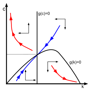
The two coupled differential equations for and form the Ramsey–Cass–Koopmans dynamical system.

![{\displaystyle {\begin{cases}{\dot {k}}=f(k)-(n+\delta )k-c\\{\dot {c}}=\sigma (c)\left[f_{k}(k)-\delta -\rho \right]\cdot c\end{cases}}}](https://wikimedia.org/api/rest_v1/media/math/render/svg/0c2d385546bae1aec2024275b8a9a4e1686b4fe6)
A steady state for the system is found by setting and equal to zero. There are three solutions:


The first is the only solution in the interior of the upper quadrant. It is a saddle point (as shown below). The second is a repelling point. The third is a degenerate stable equilibrium.
By default, the first solution is meant, although the other two solutions are important to keep track of.
Any optimal trajectory must follow the dynamical system. However, since the variable is a control variable, at each capital intensity , to find its corresponding optimal trajectory, we still need to find its starting consumption rate . As it turns out, the optimal trajectory is the unique one that converges to the interior equilibrium point. Any other trajectory either converges to the all-saving equilibrium with , or diverges to , which means that the economy expends all its capital in finite time. Both achieve a lower overall utility than the trajectory towards the interior equilibrium point.


A qualitative statement about the stability of the solution requires a linearization by a first-order Taylor polynomial

where is the Jacobian matrix evaluated at steady state,[note 5] given by


which has determinant since , is positive by assumption, and since is concave (Inada condition). Since the determinant equals the product of the eigenvalues, the eigenvalues must be real and opposite in sign.[6]


Hence by the stable manifold theorem, the equilibrium is a saddle point and there exists a unique stable arm, or “saddle path”, that converges on the equilibrium, indicated by the blue curve in the phase diagram.
The system is called “saddle path stable” since all unstable trajectories are ruled out by the “no Ponzi scheme” condition:[7]

implying that the present value of the capital stock cannot be negative.[note 6]
History
Spear and Young re-examine the history of optimal growth during the 1950s and 1960s,[8] focusing in part on the veracity of the claimed simultaneous and independent development of Cass' "Optimum growth in an aggregative model of capital accumulation" (published in 1965 in the Review of Economic Studies), and Tjalling Koopman's "On the concept of optimal economic growth" (published in Study Week on the Econometric Approach to Development Planning, 1965, Rome: Pontifical Academy of Science).
Over their lifetimes, neither Cass nor Koopmans ever suggested that their results characterizing optimal growth in the one-sector, continuous-time growth model were anything other than "simultaneous and independent". That the issue of priority ever became a discussion point was due only to the fact that in the published version of Koopmans' work, he cited the chapter from Cass' thesis that later became the RES paper. In his paper, Koopmans states in a footnote that Cass independently obtained conditions similar to what Koopmans finds, and that Cass also considers the limiting case where the discount rate goes to zero in his paper. For his part, Cass notes that "after the original version of this paper was completed, a very similar analysis by Koopmans came to our attention. We draw on his results in discussing the limiting case, where the effective social discount rate goes to zero". In the interview that Cass gave to Macroeconomic Dynamics, he credits Koopmans with pointing him to Frank Ramsey's previous work, claiming to have been embarrassed not to have known of it, but says nothing to dispel the basic claim that his work and Koopmans' were in fact independent.
Spear and Young dispute this history, based upon a previously overlooked working paper version of Koopmans' paper,[9] which was the basis for Koopmans' oft-cited presentation at a conference held by the Pontifical Academy of Sciences in October 1963.[10] In this Cowles Discussion paper, there is an error. Koopmans claims in his main result that the Euler equations are both necessary and sufficient to characterize optimal trajectories in the model because any solutions to the Euler equations which do not converge to the optimal steady-state would hit either a zero consumption or zero capital boundary in finite time. This error was apparently presented at the Vatican conference, although at the time of Koopmans' presenting it, no participant commented on the problem. This can be inferred because the discussion after each paper presentation at the Vatican conference is preserved verbatim in the conference volume.
In the Vatican volume discussion following the presentation of a paper by Edmond Malinvaud, the issue does arise because of Malinvaud's explicit inclusion of a so-called "transversality condition" (which Malinvaud calls Condition I) in his paper. At the end of the presentation, Koopmans asks Malinvaud whether it is not the case that Condition I simply guarantees that solutions to the Euler equations that do not converge to the optimal steady-state hit a boundary in finite time. Malinvaud replies that this is not the case, and suggests that Koopmans look at the example with log utility functions and Cobb-Douglas production functions.
At this point, Koopmans obviously recognizes he has a problem, but, based on a confusing appendix to a later version of the paper produced after the Vatican conference, he seems unable to decide how to deal with the issue raised by Malinvaud's Condition I.
From the Macroeconomic Dynamics interview with Cass, it is clear that Koopmans met with Cass' thesis advisor, Hirofumi Uzawa, at the winter meetings of the Econometric Society in January 1964, where Uzawa advised him that his student [Cass] had solved this problem already. Uzawa must have then provided Koopmans with the copy of Cass' thesis chapter, which he apparently sent along in the guise of the IMSSS Technical Report that Koopmans cited in the published version of his paper. The word "guise" is appropriate here, because the TR number listed in Koopmans' citation would have put the issue date of the report in the early 1950s, which it clearly was not.
In the published version of Koopmans' paper, he imposes a new Condition Alpha in addition to the Euler equations, stating that the only admissible trajectories among those satisfying the Euler equations is the one that converges to the optimal steady-state equilibrium of the model. This result is derived in Cass' paper via the imposition of a transversality condition that Cass deduced from relevant sections of a book by Lev Pontryagin.[11] Spear and Young conjecture that Koopmans took this route because he did not want to appear to be "borrowing" either Malinvaud's or Cass' transversality technology.
Based on this and other examination of Malinvaud's contributions in 1950s—specifically his intuition of the importance of the transversality condition—Spear and Young suggest that the neo-classical growth model might better be called the Ramsey–Malinvaud–Cass model than the established Ramsey–Cass–Koopmans honorific.
Notes
- ^ This result is due not just to the endogeneity of the saving rate but also because of the infinite nature of the planning horizon of the agents in the model; it does not hold in other models with endogenous saving rates but more complex intergenerational dynamics, for example, in Samuelson's or Diamond's overlapping generations models.
- ^ The assumption that is in fact crucial for the analysis. If , then for low values of the optimal value of is 0 and therefore if is sufficiently low there exists an initial time interval where even if , see Nævdal, E. (2019). "New Insights From The Canonical Ramsey–Cass–Koopmans Growth Model". Macroeconomic Dynamics. 25 (6): 1569–1577. doi:10.1017/S1365100519000786. S2CID 214268940.
- ^ The Hamiltonian for the Ramsey–Cass–Koopmans problem is
- ^ The problem can also be solved with classical calculus of variations methods, see Hadley, G.; Kemp, M. C. (1971). Variational Methods in Economics. New York: Elsevier. pp. 50–71. ISBN 978-0-444-10097-9.
- ^ The Jacobian matrix of the Ramsey–Cass–Koopmans system is
- ^ It can be shown that the “no Ponzi scheme” condition follows from the transversality condition on the Hamiltonian, see Barro, Robert J.; Sala-i-Martin, Xavier (2004). Economic Growth (Second ed.). New York: McGraw-Hill. pp. 91–92. ISBN 978-0-262-02553-9.


![{\displaystyle H=e^{-\rho t}u(c)+\mu \left[f(k)-(n+\delta )k-c\right]}](https://wikimedia.org/api/rest_v1/media/math/render/svg/63ca47c8d8e4ce7f389e1e11f4696fcabc803319)


![{\displaystyle \mathbf {J} \left(k,c\right)={\begin{bmatrix}{\frac {\partial {\dot {k}}}{\partial k}}&{\frac {\partial {\dot {k}}}{\partial c}}\\{\frac {\partial {\dot {c}}}{\partial k}}&{\frac {\partial {\dot {c}}}{\partial c}}\end{bmatrix}}={\begin{bmatrix}f_{k}(k)-(n+\delta )&-1\\{\frac {1}{\sigma }}f_{kk}(k)\cdot c&{\frac {1}{\sigma }}\left[f_{k}(k)-\delta -\rho \right]\end{bmatrix}}}](https://wikimedia.org/api/rest_v1/media/math/render/svg/f7d33d5204abc754b93f17a3c5ff091f4135cdf5)
References
- ^ Ramsey, Frank P. (1928). "A Mathematical Theory of Saving". Economic Journal. 38 (152): 543–559. doi:10.2307/2224098. JSTOR 2224098.
- ^ Cass, David (1965). "Optimum Growth in an Aggregative Model of Capital Accumulation". Review of Economic Studies. 32 (3): 233–240. doi:10.2307/2295827. JSTOR 2295827.
- ^ Koopmans, T. C. (1965). "On the Concept of Optimal Economic Growth". The Economic Approach to Development Planning. Chicago: Rand McNally. pp. 225–287.
- ^ Collard, David A. (2011). "Ramsey, saving and the generations". Generations of Economists. London: Routledge. pp. 256–273. ISBN 978-0-415-56541-7.
- ^ Blanchard, Olivier Jean; Fischer, Stanley (1989). Lectures on Macroeconomics. Cambridge: MIT Press. pp. 41–43. ISBN 978-0-262-02283-5.
- ^ Beavis, Brian; Dobbs, Ian (1990). Optimization and Stability Theory for Economic Analysis. New York: Cambridge University Press. p. 157. ISBN 978-0-521-33605-5.
- ^ Roe, Terry L.; Smith, Rodney B. W.; Saracoglu, D. Sirin (2009). Multisector Growth Models: Theory and Application. New York: Springer. p. 48. ISBN 978-0-387-77358-2.
- ^ Spear, S. E.; Young, W. (2014). "Optimum Savings and Optimal Growth: The Cass–Malinvaud–Koopmans Nexus". Macroeconomic Dynamics. 18 (1): 215–243. doi:10.1017/S1365100513000291. S2CID 1340808.
- ^ Koopmans, Tjalling (December 1963). "On the Concept of Optimal Economic Growth" (PDF). Cowles Foundation Discussion Paper 163.
- ^ McKenzie, Lionel (2002). "Some Early Conferences on Growth Theory". In Bitros, George; Katsoulacos, Yannis (eds.). Essays in Economic Theory, Growth and Labor Markets. Cheltenham: Edward Elgar. pp. 3–18. ISBN 978-1-84064-739-6.
- ^ Pontryagin, Lev; Boltyansky, Vladimir; Gamkrelidze, Revaz; Mishchenko, Evgenii (1962). The Mathematical Theory of Optimal Processes. New York: John Wiley.
Further reading
- Acemoglu, Daron (2009). "The Neoclassical Growth Model". Introduction to Modern Economic Growth. Princeton: Princeton University Press. pp. 287–326. ISBN 978-0-691-13292-1.
- Barro, Robert J.; Sala-i-Martin, Xavier (2004). "Growth Models with Consumer Optimization". Economic Growth (Second ed.). New York: McGraw-Hill. pp. 85–142. ISBN 978-0-262-02553-9.
- Bénassy, Jean-Pascal (2011). "The Ramsey Model". Macroeconomic Theory. New York: Oxford University Press. pp. 145–160. ISBN 978-0-19-538771-1.
- Blanchard, Olivier Jean; Fischer, Stanley (1989). "Consumption and Investment: Basic Infinite Horizon Models". Lectures on Macroeconomics. Cambridge: MIT Press. pp. 37–89. ISBN 978-0-262-02283-5.
- Miao, Jianjun (2014). "Neoclassical Growth Models". Economic Dynamics in Discrete Time. Cambridge: MIT Press. pp. 353–364. ISBN 978-0-262-02761-8.
- Novales, Alfonso; Fernández, Esther; Ruíz, Jesús (2009). "Optimal Growth: Continuous Time Analysis". Economic Growth: Theory and Numerical Solution Methods. Berlin: Springer. pp. 101–154. ISBN 978-3-540-68665-1.
- Romer, David (2011). "Infinite-Horizon and Overlapping-Generations Models". Advanced Macroeconomics (Fourth ed.). New York: McGraw-Hill. pp. 49–77. ISBN 978-0-07-351137-5.