

Radiocarbon dating (also referred to as carbon dating or carbon-14 dating) is a method for determining the age of an object containing organic material by using the properties of radiocarbon, a radioactive isotope of carbon.
The method was developed in the late 1940s at the University of Chicago by Willard Libby. It is based on the fact that radiocarbon (14
C) is constantly being created in the Earth's atmosphere by the interaction of cosmic rays with atmospheric nitrogen. The resulting 14
C combines with atmospheric oxygen to form radioactive carbon dioxide, which is incorporated into plants by photosynthesis; animals then acquire 14
C by eating the plants. When the animal or plant dies, it stops exchanging carbon with its environment, and thereafter the amount of 14
C it contains begins to decrease as the 14
C undergoes radioactive decay. Measuring the proportion of 14
C in a sample from a dead plant or animal, such as a piece of wood or a fragment of bone, provides information that can be used to calculate when the animal or plant died. The older a sample is, the less 14
C there is to be detected, and because the half-life of 14
C (the period of time after which half of a given sample will have decayed) is about 5,730 years, the oldest dates that can be reliably measured by this process date to approximately 50,000 years ago (in this interval about 99.8% of the 14
C will have decayed), although special preparation methods occasionally make an accurate analysis of older samples possible. In 1960, Libby received the Nobel Prize in Chemistry for his work.
Research has been ongoing since the 1960s to determine what the proportion of 14
C in the atmosphere has been over the past 50,000 years. The resulting data, in the form of a calibration curve, is now used to convert a given measurement of radiocarbon in a sample into an estimate of the sample's calendar age. Other corrections must be made to account for the proportion of 14
C in different types of organisms (fractionation), and the varying levels of 14
C throughout the biosphere (reservoir effects). Additional complications come from the burning of fossil fuels such as coal and oil, and from the above-ground nuclear tests performed in the 1950s and 1960s.
Because the time it takes to convert biological materials to fossil fuels is substantially longer than the time it takes for its 14
C to decay below detectable levels, fossil fuels contain almost no 14
C. As a result, beginning in the late 19th century, there was a noticeable drop in the proportion of 14
C in the atmosphere as the carbon dioxide generated from burning fossil fuels began to accumulate. Conversely, nuclear testing increased the amount of 14
C in the atmosphere, which reached a maximum in about 1965 of almost double the amount present in the atmosphere prior to nuclear testing.
Measurement of radiocarbon was originally done with beta-counting devices, which counted the amount of beta radiation emitted by decaying 14
C atoms in a sample. More recently, accelerator mass spectrometry has become the method of choice; it counts all the 14
C atoms in the sample and not just the few that happen to decay during the measurements; it can therefore be used with much smaller samples (as small as individual plant seeds), and gives results much more quickly. The development of radiocarbon dating has had a profound impact on archaeology. In addition to permitting more accurate dating within archaeological sites than previous methods, it allows comparison of dates of events across great distances. Histories of archaeology often refer to its impact as the "radiocarbon revolution". Radiocarbon dating has allowed key transitions in prehistory to be dated, such as the end of the last ice age, and the beginning of the Neolithic and Bronze Age in different regions.
YouTube Encyclopedic
-
1/5Views:457 73221 164368 841162 0713 249 302
-
How to Date a Dead Thing
-
Carbon-14 dating | The Day Tomorrow Began
-
Why Carbon Dating Might Be in Danger
-
Radiocarbon Dating
-
Not All Carbon is Radiocarbon
Transcription
Background
History
In 1939, Martin Kamen and Samuel Ruben of the Radiation Laboratory at Berkeley began experiments to determine if any of the elements common in organic matter had isotopes with half-lives long enough to be of value in biomedical research. They synthesized 14
C using the laboratory's cyclotron accelerator and soon discovered that the atom's half-life was far longer than had been previously thought.[1] This was followed by a prediction by Serge A. Korff, then employed at the Franklin Institute in Philadelphia, that the interaction of thermal neutrons with 14
N in the upper atmosphere would create 14
C.[note 1][3][4] It had previously been thought that 14
C would be more likely to be created by deuterons interacting with 13
C.[1] At some time during World War II, Willard Libby, who was then at Berkeley, learned of Korff's research and conceived the idea that it might be possible to use radiocarbon for dating.[3][4]
In 1945, Libby moved to the University of Chicago, where he began his work on radiocarbon dating. He published a paper in 1946 in which he proposed that the carbon in living matter might include 14
C as well as non-radioactive carbon.[5][6] Libby and several collaborators proceeded to experiment with methane collected from sewage works in Baltimore, and after isotopically enriching their samples they were able to demonstrate that they contained 14
C. By contrast, methane created from petroleum showed no radiocarbon activity because of its age. The results were summarized in a paper in Science in 1947, in which the authors commented that their results implied it would be possible to date materials containing carbon of organic origin.[5][7]
Libby and James Arnold proceeded to test the radiocarbon dating theory by analyzing samples with known ages. For example, two samples taken from the tombs of two Egyptian kings, Zoser and Sneferu, independently dated to 2625 BC plus or minus 75 years, were dated by radiocarbon measurement to an average of 2800 BC plus or minus 250 years. These results were published in Science in December 1949.[8][9][note 2] Within 11 years of their announcement, more than 20 radiocarbon dating laboratories had been set up worldwide.[11] In 1960, Libby was awarded the Nobel Prize in Chemistry for this work.[5]
Physical and chemical details
In nature, carbon exists as three isotopes: two stable, nonradioactive (carbon-12 (12
C), and carbon-13 (13
C), and one radioactive carbon-14 (14
C), also known as "radiocarbon"). The half-life of 14
C (the time it takes for half of a given amount of 14
C to decay) is about 5,730 years, so its concentration in the atmosphere might be expected to decrease over thousands of years, but 14
C is constantly being produced in the lower stratosphere and upper troposphere, primarily by galactic cosmic rays, and to a lesser degree by solar cosmic rays.[5][12] These cosmic rays generate neutrons as they travel through the atmosphere which can strike nitrogen-14 (14
N) atoms and turn them into 14
C.[5] The following nuclear reaction is the main pathway by which 14
C is created:
n + 14
7N
→ 14
6C
+ p
where n represents a neutron and p represents a proton.[13][14][note 3]
Once produced, the 14
C quickly combines with the oxygen (O) in the atmosphere to form first carbon monoxide (CO),[14] and ultimately carbon dioxide (CO
2).[15]
14C + O2 → 14CO + O
14CO + OH → 14CO2 + H
Carbon dioxide produced in this way diffuses in the atmosphere, is dissolved in the ocean, and is taken up by plants via photosynthesis. Animals eat the plants, and ultimately the radiocarbon is distributed throughout the biosphere. The ratio of 14
C to 12
C is approximately 1.25 parts of 14
C to 1012 parts of 12
C.[16] In addition, about 1% of the carbon atoms are of the stable isotope 13
C.[5]
The equation for the radioactive decay of 14
C is:[17]
14
6C
→ 14
7N
+
e−
+
ν
e
By emitting a beta particle (an electron, e−) and an electron antineutrino (
ν
e), one of the neutrons in the 14
C nucleus changes to a proton and the 14
C nucleus reverts to the stable (non-radioactive) isotope 14
N.[18]
Principles
During its life, a plant or animal is in equilibrium with its surroundings by exchanging carbon either with the atmosphere or through its diet. It will, therefore, have the same proportion of 14
C as the atmosphere, or in the case of marine animals or plants, with the ocean. Once it dies, it ceases to acquire 14
C, but the 14
C within its biological material at that time will continue to decay, and so the ratio of 14
C to 12
C in its remains will gradually decrease. Because 14
C decays at a known rate, the proportion of radiocarbon can be used to determine how long it has been since a given sample stopped exchanging carbon – the older the sample, the less 14
C will be left.[16]
The equation governing the decay of a radioactive isotope is:[5]

where N0 is the number of atoms of the isotope in the original sample (at time t = 0, when the organism from which the sample was taken died), and N is the number of atoms left after time t.[5] λ is a constant that depends on the particular isotope; for a given isotope it is equal to the reciprocal of the mean-life – i.e. the average or expected time a given atom will survive before undergoing radioactive decay.[5] The mean-life, denoted by τ, of 14
C is 8,267 years,[note 4] so the equation above can be rewritten as:[20]

The sample is assumed to have originally had the same 14
C/12
C ratio as the ratio in the atmosphere, and since the size of the sample is known, the total number of atoms in the sample can be calculated, yielding N0, the number of 14
C atoms in the original sample. Measurement of N, the number of 14
C atoms currently in the sample, allows the calculation of t, the age of the sample, using the equation above.[16]
The half-life of a radioactive isotope (usually denoted by t1/2) is a more familiar concept than the mean-life, so although the equations above are expressed in terms of the mean-life, it is more usual to quote the value of 14
C's half-life than its mean-life. The currently accepted value for the half-life of 14
C is 5,700 ± 30 years.[21] This means that after 5,700 years, only half of the initial 14
C will remain; a quarter will remain after 11,400 years; an eighth after 17,100 years; and so on.
The above calculations make several assumptions, such as that the level of 14
C in the atmosphere has remained constant over time.[5] In fact, the level of 14
C in the atmosphere has varied significantly and as a result, the values provided by the equation above have to be corrected by using data from other sources.[22] This is done by calibration curves (discussed below), which convert a measurement of 14
C in a sample into an estimated calendar age. The calculations involve several steps and include an intermediate value called the "radiocarbon age", which is the age in "radiocarbon years" of the sample: an age quoted in radiocarbon years means that no calibration curve has been used − the calculations for radiocarbon years assume that the atmospheric 14
C/12
C ratio has not changed over time.[23][24]
Calculating radiocarbon ages also requires the value of the half-life for 14
C. In Libby's 1949 paper he used a value of 5720 ± 47 years, based on research by Engelkemeir et al.[25] This was remarkably close to the modern value, but shortly afterwards the accepted value was revised to 5568 ± 30 years,[26] and this value was in use for more than a decade. It was revised again in the early 1960s to 5,730 ± 40 years,[27][28] which meant that many calculated dates in papers published prior to this were incorrect (the error in the half-life is about 3%).[note 5] For consistency with these early papers, it was agreed at the 1962 Radiocarbon Conference in Cambridge (UK) to use the "Libby half-life" of 5568 years. Radiocarbon ages are still calculated using this half-life, and are known as "Conventional Radiocarbon Age". Since the calibration curve (IntCal) also reports past atmospheric 14
C concentration using this conventional age, any conventional ages calibrated against the IntCal curve will produce a correct calibrated age. When a date is quoted, the reader should be aware that if it is an uncalibrated date (a term used for dates given in radiocarbon years) it may differ substantially from the best estimate of the actual calendar date, both because it uses the wrong value for the half-life of 14
C, and because no correction (calibration) has been applied for the historical variation of 14
C in the atmosphere over time.[23][24][30][note 6]
Carbon exchange reservoir

C in each reservoir[5][note 7]
Carbon is distributed throughout the atmosphere, the biosphere, and the oceans; these are referred to collectively as the carbon exchange reservoir,[33] and each component is also referred to individually as a carbon exchange reservoir. The different elements of the carbon exchange reservoir vary in how much carbon they store, and in how long it takes for the 14
C generated by cosmic rays to fully mix with them. This affects the ratio of 14
C to 12
C in the different reservoirs, and hence the radiocarbon ages of samples that originated in each reservoir.[5] The atmosphere, which is where 14
C is generated, contains about 1.9% of the total carbon in the reservoirs, and the 14
C it contains mixes in less than seven years.[34] The ratio of 14
C to 12
C in the atmosphere is taken as the baseline for the other reservoirs: if another reservoir has a lower ratio of 14
C to 12
C, it indicates that the carbon is older and hence that either some of the 14
C has decayed, or the reservoir is receiving carbon that is not at the atmospheric baseline.[22] The ocean surface is an example: it contains 2.4% of the carbon in the exchange reservoir, but there is only about 95% as much 14
C as would be expected if the ratio were the same as in the atmosphere.[5] The time it takes for carbon from the atmosphere to mix with the surface ocean is only a few years,[35] but the surface waters also receive water from the deep ocean, which has more than 90% of the carbon in the reservoir.[22] Water in the deep ocean takes about 1,000 years to circulate back through surface waters, and so the surface waters contain a combination of older water, with depleted 14
C, and water recently at the surface, with 14
C in equilibrium with the atmosphere.[22]
Creatures living at the ocean surface have the same 14
C ratios as the water they live in, and as a result of the reduced 14
C/12
C ratio, the radiocarbon age of marine life is typically about 400 years.[36][37] Organisms on land are in closer equilibrium with the atmosphere and have the same 14
C/12
C ratio as the atmosphere.[5][note 8] These organisms contain about 1.3% of the carbon in the reservoir; sea organisms have a mass of less than 1% of those on land and are not shown in the diagram. Accumulated dead organic matter, of both plants and animals, exceeds the mass of the biosphere by a factor of nearly 3, and since this matter is no longer exchanging carbon with its environment, it has a 14
C/12
C ratio lower than that of the biosphere.[5]
Dating considerations
The variation in the 14
C/12
C ratio in different parts of the carbon exchange reservoir means that a straightforward calculation of the age of a sample based on the amount of 14
C it contains will often give an incorrect result. There are several other possible sources of error that need to be considered. The errors are of four general types:
- variations in the 14
C/12
C ratio in the atmosphere, both geographically and over time; - isotopic fractionation;
- variations in the 14
C/12
C ratio in different parts of the reservoir; - contamination.
Atmospheric variation
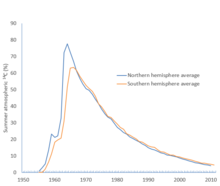
C for the northern and southern hemispheres, showing percentage excess above pre-bomb levels. The Partial Test Ban Treaty went into effect on 10 October 1963.[38]
In the early years of using the technique, it was understood that it depended on the atmospheric 14
C/12
C ratio having remained the same over the preceding few thousand years. To verify the accuracy of the method, several artefacts that were datable by other techniques were tested; the results of the testing were in reasonable agreement with the true ages of the objects. Over time, however, discrepancies began to appear between the known chronology for the oldest Egyptian dynasties and the radiocarbon dates of Egyptian artefacts. Neither the pre-existing Egyptian chronology nor the new radiocarbon dating method could be assumed to be accurate, but a third possibility was that the 14
C/12
C ratio had changed over time. The question was resolved by the study of tree rings:[39][40][41] comparison of overlapping series of tree rings allowed the construction of a continuous sequence of tree-ring data that spanned 8,000 years.[39] (Since that time the tree-ring data series has been extended to 13,900 years.)[30] In the 1960s, Hans Suess was able to use the tree-ring sequence to show that the dates derived from radiocarbon were consistent with the dates assigned by Egyptologists. This was possible because although annual plants, such as corn, have a 14
C/12
C ratio that reflects the atmospheric ratio at the time they were growing, trees only add material to their outermost tree ring in any given year, while the inner tree rings do not get their 14
C replenished and instead only lose 14
C through radioactive decay. Hence each ring preserves a record of the atmospheric 14
C/12
C ratio of the year it grew in. Carbon-dating the wood from the tree rings themselves provides the check needed on the atmospheric 14
C/12
C ratio: with a sample of known date, and a measurement of the value of N (the number of atoms of 14
C remaining in the sample), the carbon-dating equation allows the calculation of N0 – the number of atoms of 14
C in the sample at the time the tree ring was formed – and hence the 14
C/12
C ratio in the atmosphere at that time.[39][41] Equipped with the results of carbon-dating the tree rings, it became possible to construct calibration curves designed to correct the errors caused by the variation over time in the 14
C/12
C ratio.[42] These curves are described in more detail below.
Coal and oil began to be burned in large quantities during the 19th century. Both are sufficiently old that they contain little or no detectable 14
C and, as a result, the CO
2 released substantially diluted the atmospheric 14
C/12
C ratio. Dating an object from the early 20th century hence gives an apparent date older than the true date. For the same reason, 14
C concentrations in the neighbourhood of large cities are lower than the atmospheric average. This fossil fuel effect (also known as the Suess effect, after Hans Suess, who first reported it in 1955) would only amount to a reduction of 0.2% in 14
C activity if the additional carbon from fossil fuels were distributed throughout the carbon exchange reservoir, but because of the long delay in mixing with the deep ocean, the actual effect is a 3% reduction.[39][43]
A much larger effect comes from above-ground nuclear testing, which released large numbers of neutrons into the atmosphere, resulting in the creation of 14
C. From about 1950 until 1963, when atmospheric nuclear testing was banned, it is estimated that several tonnes of 14
C were created. If all this extra 14
C had immediately been spread across the entire carbon exchange reservoir, it would have led to an increase in the 14
C/12
C ratio of only a few per cent, but the immediate effect was to almost double the amount of 14
C in the atmosphere, with the peak level occurring in 1964 for the northern hemisphere, and in 1966 for the southern hemisphere. The level has since dropped, as this bomb pulse or "bomb carbon" (as it is sometimes called) percolates into the rest of the reservoir.[39][43][44][38]
Isotopic fractionation
Photosynthesis is the primary process by which carbon moves from the atmosphere into living things. In photosynthetic pathways 12
C is absorbed slightly more easily than 13
C, which in turn is more easily absorbed than 14
C. The differential uptake of the three carbon isotopes leads to 13
C/12
C and 14
C/12
C ratios in plants that differ from the ratios in the atmosphere. This effect is known as isotopic fractionation.[45][46]
To determine the degree of fractionation that takes place in a given plant, the amounts of both 12
C and 13
C isotopes are measured, and the resulting 13
C/12
C ratio is then compared to a standard ratio known as PDB.[note 9] The 13
C/12
C ratio is used instead of 14
C/12
C because the former is much easier to measure, and the latter can be easily derived: the depletion of 13
C relative to 12
C is proportional to the difference in the atomic masses of the two isotopes, so the depletion for 14
C is twice the depletion of 13
C.[22] The fractionation of 13
C, known as δ13C, is calculated as follows:[45]
‰

where the ‰ sign indicates parts per thousand.[45] Because the PDB standard contains an unusually high proportion of 13
C,[note 10] most measured δ13C values are negative.

| Material | Typical δ13C range |
|---|---|
| PDB | 0‰ |
| Marine plankton | −22‰ to −17‰[46] |
| C3 plants | −30‰ to −22‰[46] |
| C4 plants | −15‰ to −9‰[46] |
| Atmospheric CO 2 |
−8‰[45] |
| Marine CO 2 |
−32‰ to −13‰[46] |
For marine organisms, the details of the photosynthesis reactions are less well understood, and the δ13C values for marine photosynthetic organisms are dependent on temperature. At higher temperatures, CO
2 has poor solubility in water, which means there is less CO
2 available for the photosynthetic reactions. Under these conditions, fractionation is reduced, and at temperatures above 14 °C (57 °F) the δ13C values are correspondingly higher, while at lower temperatures, CO
2 becomes more soluble and hence more available to marine organisms.[46]
The δ13C value for animals depends on their diet. An animal that eats food with high δ13C values will have a higher δ13C than one that eats food with lower δ13C values.[45] The animal's own biochemical processes can also impact the results: for example, both bone minerals and bone collagen typically have a higher concentration of 13
C than is found in the animal's diet, though for different biochemical reasons. The enrichment of bone 13
C also implies that excreted material is depleted in 13
C relative to the diet.[49]
Since 13
C makes up about 1% of the carbon in a sample, the 13
C/12
C ratio can be accurately measured by mass spectrometry.[22] Typical values of δ13C have been found by experiment for many plants, as well as for different parts of animals such as bone collagen, but when dating a given sample it is better to determine the δ13C value for that sample directly than to rely on the published values.[45]
The carbon exchange between atmospheric CO
2 and carbonate at the ocean surface is also subject to fractionation, with 14
C in the atmosphere more likely than 12
C to dissolve in the ocean. The result is an overall increase in the 14
C/12
C ratio in the ocean of 1.5%, relative to the 14
C/12
C ratio in the atmosphere. This increase in 14
C concentration almost exactly cancels out the decrease caused by the upwelling of water (containing old, and hence 14
C-depleted, carbon) from the deep ocean, so that direct measurements of 14
C radiation are similar to measurements for the rest of the biosphere. Correcting for isotopic fractionation, as is done for all radiocarbon dates to allow comparison between results from different parts of the biosphere, gives an apparent age of about 400 years for ocean surface water.[22][37]
Reservoir effects
Libby's original exchange reservoir hypothesis assumed that the 14
C/12
C ratio in the exchange reservoir is constant all over the world,[50] but it has since been discovered that there are several causes of variation in the ratio across the reservoir.[36]
Marine effect
The CO
2 in the atmosphere transfers to the ocean by dissolving in the surface water as carbonate and bicarbonate ions; at the same time the carbonate ions in the water are returning to the air as CO
2.[50] This exchange process brings 14
C from the atmosphere into the surface waters of the ocean, but the 14
C thus introduced takes a long time to percolate through the entire volume of the ocean. The deepest parts of the ocean mix very slowly with the surface waters, and the mixing is uneven. The main mechanism that brings deep water to the surface is upwelling, which is more common in regions closer to the equator. Upwelling is also influenced by factors such as the topography of the local ocean bottom and coastlines, the climate, and wind patterns. Overall, the mixing of deep and surface waters takes far longer than the mixing of atmospheric CO
2 with the surface waters, and as a result water from some deep ocean areas has an apparent radiocarbon age of several thousand years. Upwelling mixes this "old" water with the surface water, giving the surface water an apparent age of about several hundred years (after correcting for fractionation).[36] This effect is not uniform – the average effect is about 400 years, but there are local deviations of several hundred years for areas that are geographically close to each other.[36][37] These deviations can be accounted for in calibration, and users of software such as CALIB can provide as an input the appropriate correction for the location of their samples.[15] The effect also applies to marine organisms such as shells, and marine mammals such as whales and seals, which have radiocarbon ages that appear to be hundreds of years old.[36]
Hemisphere effect
The northern and southern hemispheres have atmospheric circulation systems that are sufficiently independent of each other that there is a noticeable time lag in mixing between the two. The atmospheric 14
C/12
C ratio is lower in the southern hemisphere, with an apparent additional age of about 40 years for radiocarbon results from the south as compared to the north.[note 11] This is because the greater surface area of ocean in the southern hemisphere means that there is more carbon exchanged between the ocean and the atmosphere than in the north. Since the surface ocean is depleted in 14
C because of the marine effect, 14
C is removed from the southern atmosphere more quickly than in the north.[36][51] The effect is strengthened by strong upwelling around Antarctica.[12]
Other effects
If the carbon in freshwater is partly acquired from aged carbon, such as rocks, then the result will be a reduction in the 14
C/12
C ratio in the water. For example, rivers that pass over limestone, which is mostly composed of calcium carbonate, will acquire carbonate ions. Similarly, groundwater can contain carbon derived from the rocks through which it has passed. These rocks are usually so old that they no longer contain any measurable 14
C, so this carbon lowers the 14
C/12
C ratio of the water it enters, which can lead to apparent ages of thousands of years for both the affected water and the plants and freshwater organisms that live in it.[22] This is known as the hard water effect because it is often associated with calcium ions, which are characteristic of hard water; other sources of carbon such as humus can produce similar results, and can also reduce the apparent age if they are of more recent origin than the sample.[36] The effect varies greatly and there is no general offset that can be applied; additional research is usually needed to determine the size of the offset, for example by comparing the radiocarbon age of deposited freshwater shells with associated organic material.[52]
Volcanic eruptions eject large amounts of carbon into the air. The carbon is of geological origin and has no detectable 14
C, so the 14
C/12
C ratio in the vicinity of the volcano is depressed relative to surrounding areas. Dormant volcanoes can also emit aged carbon. Plants that photosynthesize this carbon also have lower 14
C/12
C ratios: for example, plants in the neighbourhood of the Furnas caldera in the Azores were found to have apparent ages that ranged from 250 years to 3320 years.[53]
Contamination
Any addition of carbon to a sample of a different age will cause the measured date to be inaccurate. Contamination with modern carbon causes a sample to appear to be younger than it really is: the effect is greater for older samples. If a sample that is 17,000 years old is contaminated so that 1% of the sample is modern carbon, it will appear to be 600 years younger; for a sample that is 34,000 years old, the same amount of contamination would cause an error of 4,000 years. Contamination with old carbon, with no remaining 14
C, causes an error in the other direction independent of age – a sample contaminated with 1% old carbon will appear to be about 80 years older than it truly is, regardless of the date of the sample.[54]
Samples
Samples for dating need to be converted into a form suitable for measuring the 14
C content; this can mean conversion to gaseous, liquid, or solid form, depending on the measurement technique to be used. Before this can be done, the sample must be treated to remove any contamination and any unwanted constituents.[55] This includes removing visible contaminants, such as rootlets that may have penetrated the sample since its burial.[55] Alkali and acid washes can be used to remove humic acid and carbonate contamination, but care has to be taken to avoid removing the part of the sample that contains the carbon to be tested.[56]
Material considerations
- It is common to reduce a wood sample to just the cellulose component before testing, but since this can reduce the volume of the sample to 20% of its original size, testing of the whole wood is often performed as well. Charcoal is often tested but is likely to need treatment to remove contaminants.[55][56]
- Unburnt bone can be tested; it is usual to date it using collagen, the protein fraction that remains after washing away the bone's structural material. Hydroxyproline, one of the constituent amino acids in bone, was once thought to be a reliable indicator as it was not known to occur except in bone, but it has since been detected in groundwater.[55]
- For burnt bone, testability depends on the conditions under which the bone was burnt. If the bone was heated under reducing conditions, it (and associated organic matter) may have been carbonized. In this case, the sample is often usable.[55]
- Shells from both marine and land organisms consist almost entirely of calcium carbonate, either as aragonite or as calcite, or some mixture of the two. Calcium carbonate is very susceptible to dissolving and recrystallizing; the recrystallized material will contain carbon from the sample's environment, which may be of geological origin. If testing recrystallized shell is unavoidable, it is sometimes possible to identify the original shell material from a sequence of tests.[57] It is also possible to test conchiolin, an organic protein found in shell, but it constitutes only 1–2% of shell material.[56]
- The three major components of peat are humic acid, humins, and fulvic acid. Of these, humins give the most reliable date as they are insoluble in alkali and less likely to contain contaminants from the sample's environment.[56] A particular difficulty with dried peat is the removal of rootlets, which are likely to be hard to distinguish from the sample material.[55]
- Soil contains organic material, but because of the likelihood of contamination by humic acid of more recent origin, it is very difficult to get satisfactory radiocarbon dates. It is preferable to sieve the soil for fragments of organic origin, and date the fragments with methods that are tolerant of small sample sizes.[56]
- Other materials that have been successfully dated include ivory, paper, textiles, individual seeds and grains, straw from within mud bricks, and charred food remains found in pottery.[56]
Preparation and size
Particularly for older samples, it may be useful to enrich the amount of 14
C in the sample before testing. This can be done with a thermal diffusion column. The process takes about a month and requires a sample about ten times as large as would be needed otherwise, but it allows more precise measurement of the 14
C/12
C ratio in old material and extends the maximum age that can be reliably reported.[58]
Once contamination has been removed, samples must be converted to a form suitable for the measuring technology to be used.[59] Where gas is required, CO
2 is widely used.[59][60] For samples to be used in liquid scintillation counters, the carbon must be in liquid form; the sample is typically converted to benzene. For accelerator mass spectrometry, solid graphite targets are the most common, although gaseous CO
2 can also be used.[59][61]
The quantity of material needed for testing depends on the sample type and the technology being used. There are two types of testing technology: detectors that record radioactivity, known as beta counters, and accelerator mass spectrometers. For beta counters, a sample weighing at least 10 grams (0.35 ounces) is typically required.[59] Accelerator mass spectrometry is much more sensitive, and samples containing as little as 0.5 milligrams of carbon can be used.[62]
Measurement and results

C is now most commonly done with an accelerator mass spectrometer
For decades after Libby performed the first radiocarbon dating experiments, the only way to measure the 14
C in a sample was to detect the radioactive decay of individual carbon atoms.[59] In this approach, what is measured is the activity, in number of decay events per unit mass per time period, of the sample.[60] This method is also known as "beta counting", because it is the beta particles emitted by the decaying 14
C atoms that are detected.[63] In the late 1970s an alternative approach became available: directly counting the number of 14
C and 12
C atoms in a given sample, via accelerator mass spectrometry, usually referred to as AMS.[59] AMS counts the 14
C/12
C ratio directly, instead of the activity of the sample, but measurements of activity and 14
C/12
C ratio can be converted into each other exactly.[60] For some time, beta counting methods were more accurate than AMS, but AMS is now more accurate and has become the method of choice for radiocarbon measurements.[64][65] In addition to improved accuracy, AMS has two further significant advantages over beta counting: it can perform accurate testing on samples much too small for beta counting, and it is much faster – an accuracy of 1% can be achieved in minutes with AMS, which is far quicker than would be achievable with the older technology.[66]
Beta counting
Libby's first detector was a Geiger counter of his own design. He converted the carbon in his sample to lamp black (soot) and coated the inner surface of a cylinder with it. This cylinder was inserted into the counter in such a way that the counting wire was inside the sample cylinder, in order that there should be no material between the sample and the wire.[59] Any interposing material would have interfered with the detection of radioactivity, since the beta particles emitted by decaying 14
C are so weak that half are stopped by a 0.01 mm (0.00039 in) thickness of aluminium.[60]
Libby's method was soon superseded by gas proportional counters, which were less affected by bomb carbon (the additional 14
C created by nuclear weapons testing). These counters record bursts of ionization caused by the beta particles emitted by the decaying 14
C atoms; the bursts are proportional to the energy of the particle, so other sources of ionization, such as background radiation, can be identified and ignored. The counters are surrounded by lead or steel shielding, to eliminate background radiation and to reduce the incidence of cosmic rays. In addition, anticoincidence detectors are used; these record events outside the counter and any event recorded simultaneously both inside and outside the counter is regarded as an extraneous event and ignored.[60]
The other common technology used for measuring 14
C activity is liquid scintillation counting, which was invented in 1950, but which had to wait until the early 1960s, when efficient methods of benzene synthesis were developed, to become competitive with gas counting; after 1970 liquid counters became the more common technology choice for newly constructed dating laboratories. The counters work by detecting flashes of light caused by the beta particles emitted by 14
C as they interact with a fluorescing agent added to the benzene. Like gas counters, liquid scintillation counters require shielding and anticoincidence counters.[67][68]
For both the gas proportional counter and liquid scintillation counter, what is measured is the number of beta particles detected in a given time period. Since the mass of the sample is known, this can be converted to a standard measure of activity in units of either counts per minute per gram of carbon (cpm/g C), or becquerels per kg (Bq/kg C, in SI units). Each measuring device is also used to measure the activity of a blank sample – a sample prepared from carbon old enough to have no activity. This provides a value for the background radiation, which must be subtracted from the measured activity of the sample being dated to get the activity attributable solely to that sample's 14
C. In addition, a sample with a standard activity is measured, to provide a baseline for comparison.[69]
Accelerator mass spectrometry

AMS counts the atoms of 14
C and 12
C in a given sample, determining the 14
C/12
C ratio directly. The sample, often in the form of graphite, is made to emit C− ions (carbon atoms with a single negative charge), which are injected into an accelerator. The ions are accelerated and passed through a stripper, which removes several electrons so that the ions emerge with a positive charge. The ions, which may have from 1 to 4 positive charges (C+ to C4+), depending on the accelerator design, are then passed through a magnet that curves their path; the heavier ions are curved less than the lighter ones, so the different isotopes emerge as separate streams of ions. A particle detector then records the number of ions detected in the 14
C stream, but since the volume of 12
C (and 13
C, needed for calibration) is too great for individual ion detection, counts are determined by measuring the electric current created in a Faraday cup.[70] The large positive charge induced by the stripper forces molecules such as 13
CH, which has a weight close enough to 14
C to interfere with the measurements, to dissociate, so they are not detected.[71] Most AMS machines also measure the sample's δ13C, for use in calculating the sample's radiocarbon age.[72] The use of AMS, as opposed to simpler forms of mass spectrometry, is necessary because of the need to distinguish the carbon isotopes from other atoms or molecules that are very close in mass, such as 14
N and 13
CH.[59] As with beta counting, both blank samples and standard samples are used.[70] Two different kinds of blank may be measured: a sample of dead carbon that has undergone no chemical processing, to detect any machine background, and a sample known as a process blank made from dead carbon that is processed into target material in exactly the same way as the sample which is being dated. Any 14
C signal from the machine background blank is likely to be caused either by beams of ions that have not followed the expected path inside the detector or by carbon hydrides such as 12
CH
2 or 13
CH. A 14
C signal from the process blank measures the amount of contamination introduced during the preparation of the sample. These measurements are used in the subsequent calculation of the age of the sample.[73]
Calculations
The calculations to be performed on the measurements taken depend on the technology used, since beta counters measure the sample's radioactivity whereas AMS determines the ratio of the three different carbon isotopes in the sample.[73]
To determine the age of a sample whose activity has been measured by beta counting, the ratio of its activity to the activity of the standard must be found. To determine this, a blank sample (of old, or dead, carbon) is measured, and a sample of known activity is measured. The additional samples allow errors such as background radiation and systematic errors in the laboratory setup to be detected and corrected for.[69] The most common standard sample material is oxalic acid, such as the HOxII standard, 1,000 lb (450 kg) of which was prepared by the National Institute of Standards and Technology (NIST) in 1977 from French beet harvests.[74][75]
The results from AMS testing are in the form of ratios of 12
C, 13
C, and 14
C, which are used to calculate Fm, the "fraction modern". This is defined as the ratio between the 14
C/12
C ratio in the sample and the 14
C/12
C ratio in modern carbon, which is in turn defined as the 14
C/12
C ratio that would have been measured in 1950 had there been no fossil fuel effect.[73]
Both beta counting and AMS results have to be corrected for fractionation. This is necessary because different materials of the same age, which because of fractionation have naturally different 14
C/12
C ratios, will appear to be of different ages because the 14
C/12
C ratio is taken as the indicator of age. To avoid this, all radiocarbon measurements are converted to the measurement that would have been seen had the sample been made of wood, which has a known δ13
C value of −25‰.[23]
Once the corrected 14
C/12
C ratio is known, a "radiocarbon age" is calculated using:[76]

The calculation uses 8,033 years, the mean-life derived from Libby's half-life of 5,568 years, not 8,267 years, the mean-life derived from the more accurate modern value of 5,730 years. Libby's value for the half-life is used to maintain consistency with early radiocarbon testing results; calibration curves include a correction for this, so the accuracy of final reported calendar ages is assured.[76]
Errors and reliability
The reliability of the results can be improved by lengthening the testing time. For example, if counting beta decays for 250 minutes is enough to give an error of ± 80 years, with 68% confidence, then doubling the counting time to 500 minutes will allow a sample with only half as much 14
C to be measured with the same error term of 80 years.[77]
Radiocarbon dating is generally limited to dating samples no more than 50,000 years old, as samples older than that have insufficient 14
C to be measurable. Older dates have been obtained by using special sample preparation techniques, large samples, and very long measurement times. These techniques can allow measurement of dates up to 60,000 and in some cases up to 75,000 years before the present.[64]
Radiocarbon dates are generally presented with a range of one standard deviation (usually represented by the Greek letter sigma as 1σ) on either side of the mean. However, a date range of 1σ represents only a 68% confidence level, so the true age of the object being measured may lie outside the range of dates quoted. This was demonstrated in 1970 by an experiment run by the British Museum radiocarbon laboratory, in which weekly measurements were taken on the same sample for six months. The results varied widely (though consistently with a normal distribution of errors in the measurements), and included multiple date ranges (of 1σ confidence) that did not overlap with each other. The measurements included one with a range from about 4,250 to about 4,390 years ago, and another with a range from about 4,520 to about 4,690.[78]
Errors in procedure can also lead to errors in the results. If 1% of the benzene in a modern reference sample accidentally evaporates, scintillation counting will give a radiocarbon age that is too young by about 80 years.[79]
Calibration

The calculations given above produce dates in radiocarbon years: i.e. dates that represent the age the sample would be if the 14
C/12
C ratio had been constant historically.[80] Although Libby had pointed out as early as 1955 the possibility that this assumption was incorrect, it was not until discrepancies began to accumulate between measured ages and known historical dates for artefacts that it became clear that a correction would need to be applied to radiocarbon ages to obtain calendar dates.[81]
To produce a curve that can be used to relate calendar years to radiocarbon years, a sequence of securely dated samples is needed which can be tested to determine their radiocarbon age. The study of tree rings led to the first such sequence: individual pieces of wood show characteristic sequences of rings that vary in thickness because of environmental factors such as the amount of rainfall in a given year. These factors affect all trees in an area, so examining tree-ring sequences from old wood allows the identification of overlapping sequences. In this way, an uninterrupted sequence of tree rings can be extended far into the past. The first such published sequence, based on bristlecone pine tree rings, was created by Wesley Ferguson.[41] Hans Suess used this data to publish the first calibration curve for radiocarbon dating in 1967.[39][40][81] The curve showed two types of variation from the straight line: a long term fluctuation with a period of about 9,000 years, and a shorter-term variation, often referred to as "wiggles", with a period of decades. Suess said he drew the line showing the wiggles by "cosmic schwung", by which he meant that the variations were caused by extraterrestrial forces. It was unclear for some time whether the wiggles were real or not, but they are now well-established.[39][40][82] These short term fluctuations in the calibration curve are now known as de Vries effects, after Hessel de Vries.[83]
A calibration curve is used by taking the radiocarbon date reported by a laboratory and reading across from that date on the vertical axis of the graph. The point where this horizontal line intersects the curve will give the calendar age of the sample on the horizontal axis. This is the reverse of the way the curve is constructed: a point on the graph is derived from a sample of known age, such as a tree ring; when it is tested, the resulting radiocarbon age gives a data point for the graph.[42]
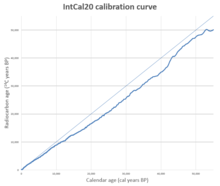
Over the next thirty years many calibration curves were published using a variety of methods and statistical approaches.[42] These were superseded by the IntCal series of curves, beginning with IntCal98, published in 1998, and updated in 2004, 2009, 2013, and 2020.[84] The improvements to these curves are based on new data gathered from tree rings, varves, coral, plant macrofossils, speleothems, and foraminifera. There are separate curves for the northern hemisphere (IntCal20) and southern hemisphere (SHCal20), as they differ systematically because of the hemisphere effect. The continuous sequence of tree-ring dates for the northern hemisphere goes back to 13,910 BP as of 2020, and this provides close to annual dating for IntCal20 much of the period, reduced where there are calibration plateaus, and increased when short term 14C spikes due to Miyake events provide additional correlation. Radiocarbon dating earlier than the continuous tree ring sequence relies on correlation with more approximate records.[85] SHCal20 is based on independent data where possible and derived from the northern curve by adding the average offset for the southern hemisphere where no direct data was available. There is also a separate marine calibration curve, MARINE20.[86][87] For a set of samples forming a sequence with a known separation in time, these samples form a subset of the calibration curve. The sequence can be compared to the calibration curve and the best match to the sequence established. This "wiggle-matching" technique can lead to more precise dating than is possible with individual radiocarbon dates.[88] Wiggle-matching can be used in places where there is a plateau on the calibration curve,[note 12] and hence can provide a much more accurate date than the intercept or probability methods are able to produce.[90] The technique is not restricted to tree rings; for example, a stratified tephra sequence in New Zealand, believed to predate human colonization of the islands, has been dated to 1314 AD ± 12 years by wiggle-matching.[91] The wiggles also mean that reading a date from a calibration curve can give more than one answer: this occurs when the curve wiggles up and down enough that the radiocarbon age intercepts the curve in more than one place, which may lead to a radiocarbon result being reported as two separate age ranges, corresponding to the two parts of the curve that the radiocarbon age intercepted.[42]
Bayesian statistical techniques can be applied when there are several radiocarbon dates to be calibrated. For example, if a series of radiocarbon dates is taken from different levels in a stratigraphic sequence, Bayesian analysis can be used to evaluate dates which are outliers and can calculate improved probability distributions, based on the prior information that the sequence should be ordered in time.[88] When Bayesian analysis was introduced, its use was limited by the need to use mainframe computers to perform the calculations, but the technique has since been implemented on programs available for personal computers, such as OxCal.[92]
Reporting dates
Several formats for citing radiocarbon results have been used since the first samples were dated. As of 2019, the standard format required by the journal Radiocarbon is as follows.[93]
Uncalibrated dates should be reported as "laboratory: year ± range BP", where:

- laboratory identifies the laboratory that tested the sample, and the sample ID
- year is the laboratory's determination of the age of the sample, in radiocarbon years
- range is the laboratory's estimate of the error in the age, at 1σ confidence.
- 'BP' stands for "before present", referring to a reference date of 1950, so that "500 BP" means the year AD 1450.
For example, the uncalibrated date "UtC-2020: 3510 ± 60 BP" indicates that the sample was tested by the Utrecht van der Graaff Laboratorium ("UtC"), where it has a sample number of "2020", and that the uncalibrated age is 3510 years before present, ± 60 years. Related forms are sometimes used: for example, "2.3 ka BP" means 2,300 radiocarbon years before present (i.e. 350 BC), and "14
C yr BP" might be used to distinguish the uncalibrated date from a date derived from another dating method such as thermoluminescence.[93]
Calibrated 14
C dates are frequently reported as "cal BP", "cal BC", or "cal AD", again with 'BP' referring to the year 1950 as the zero date.[94] Radiocarbon gives two options for reporting calibrated dates. A common format is "cal date-range confidence", where:
- date-range is the range of dates corresponding to the given confidence level
- confidence indicates the confidence level for the given date range.
For example, "cal 1220–1281 AD (1σ)" means a calibrated date for which the true date lies between AD 1220 and AD 1281, with a confidence level of '1 sigma', or approximately 68%. Calibrated dates can also be expressed as "BP" instead of using "BC" and "AD". The curve used to calibrate the results should be the latest available IntCal curve. Calibrated dates should also identify any programs, such as OxCal, used to perform the calibration.[93] In addition, an article in Radiocarbon in 2014 about radiocarbon date reporting conventions recommends that information should be provided about sample treatment, including the sample material, pretreatment methods, and quality control measurements; that the citation to the software used for calibration should specify the version number and any options or models used; and that the calibrated date should be given with the associated probabilities for each range.[95]
Use in archaeology
Interpretation
A key concept in interpreting radiocarbon dates is archaeological association: what is the true relationship between two or more objects at an archaeological site? It frequently happens that a sample for radiocarbon dating can be taken directly from the object of interest, but there are also many cases where this is not possible. Metal grave goods, for example, cannot be radiocarbon dated, but they may be found in a grave with a coffin, charcoal, or other material which can be assumed to have been deposited at the same time. In these cases, a date for the coffin or charcoal is indicative of the date of deposition of the grave goods, because of the direct functional relationship between the two. There are also cases where there is no functional relationship, but the association is reasonably strong: for example, a layer of charcoal in a rubbish pit provides a date which has a relationship to the rubbish pit.[96]
Contamination is of particular concern when dating very old material obtained from archaeological excavations and great care is needed in the specimen selection and preparation. In 2014, Thomas Higham and co-workers suggested that many of the dates published for Neanderthal artifacts are too recent because of contamination by "young carbon".[97]
As a tree grows, only the outermost tree ring exchanges carbon with its environment, so the age measured for a wood sample depends on where the sample is taken from. This means that radiocarbon dates on wood samples can be older than the date at which the tree was felled. In addition, if a piece of wood is used for multiple purposes, there may be a significant delay between the felling of the tree and the final use in the context in which it is found.[98] This is often referred to as the old wood problem.[5] One example is the Bronze Age trackway at Withy Bed Copse, in England; the trackway was built from wood that had clearly been worked for other purposes before being re-used in the trackway. Another example is driftwood, which may be used as construction material. It is not always possible to recognize re-use. Other materials can present the same problem: for example, bitumen is known to have been used by some Neolithic communities to waterproof baskets; the bitumen's radiocarbon age will be greater than is measurable by the laboratory, regardless of the actual age of the context, so testing the basket material will give a misleading age if care is not taken. A separate issue, related to re-use, is that of lengthy use, or delayed deposition. For example, a wooden object that remains in use for a lengthy period will have an apparent age greater than the actual age of the context in which it is deposited.[98]
Use outside archaeology
Archaeology is not the only field to make use of radiocarbon dating. Radiocarbon dates can also be used in geology, sedimentology, and lake studies, for example. The ability to date minute samples using AMS has meant that palaeobotanists and palaeoclimatologists can use radiocarbon dating directly on pollen purified from sediment sequences, or on small quantities of plant material or charcoal. Dates on organic material recovered from strata of interest can be used to correlate strata in different locations that appear to be similar on geological grounds. Dating material from one location gives date information about the other location, and the dates are also used to place strata in the overall geological timeline.[99]
Radiocarbon is also used to date carbon released from ecosystems, particularly to monitor the release of old carbon that was previously stored in soils as a result of human disturbance or climate change.[100] Recent advances in field collection techniques also allow the radiocarbon dating of methane and carbon dioxide, which are important greenhouse gases.[101][102]
Notable applications
Pleistocene/Holocene boundary in Two Creeks Fossil Forest
The Pleistocene is a geological epoch that began about 2.6 million years ago. The Holocene, the current geological epoch, begins about 11,700 years ago when the Pleistocene ends.[103] Establishing the date of this boundary − which is defined by sharp climatic warming − as accurately as possible has been a goal of geologists for much of the 20th century.[103][104] At Two Creeks, in Wisconsin, a fossil forest was discovered (Two Creeks Buried Forest State Natural Area), and subsequent research determined that the destruction of the forest was caused by the Valders ice readvance, the last southward movement of ice before the end of the Pleistocene in that area. Before the advent of radiocarbon dating, the fossilized trees had been dated by correlating sequences of annually deposited layers of sediment at Two Creeks with sequences in Scandinavia. This led to estimates that the trees were between 24,000 and 19,000 years old,[103] and hence this was taken to be the date of the last advance of the Wisconsin glaciation before its final retreat marked the end of the Pleistocene in North America.[105] In 1952 Libby published radiocarbon dates for several samples from the Two Creeks site and two similar sites nearby; the dates were averaged to 11,404 BP with a standard error of 350 years. This result was uncalibrated, as the need for calibration of radiocarbon ages was not yet understood. Further results over the next decade supported an average date of 11,350 BP, with the results thought to be the most accurate averaging 11,600 BP. There was initial resistance to these results on the part of Ernst Antevs, the palaeobotanist who had worked on the Scandinavian varve series, but his objections were eventually discounted by other geologists. In the 1990s samples were tested with AMS, yielding (uncalibrated) dates ranging from 11,640 BP to 11,800 BP, both with a standard error of 160 years. Subsequently, a sample from the fossil forest was used in an interlaboratory test, with results provided by over 70 laboratories. These tests produced a median age of 11,788 ± 8 BP (2σ confidence) which when calibrated gives a date range of 13,730 to 13,550 cal BP.[103] The Two Creeks radiocarbon dates are now regarded as a key result in developing the modern understanding of North American glaciation at the end of the Pleistocene.[105]
Dead Sea Scrolls

In 1947, scrolls were discovered in caves near the Dead Sea that proved to contain writing in Hebrew and Aramaic, most of which are thought to have been produced by the Essenes, a small Jewish sect. These scrolls are of great significance in the study of Biblical texts because many of them contain the earliest known version of books of the Hebrew bible.[106] A sample of the linen wrapping from one of these scrolls, the Great Isaiah Scroll, was included in a 1955 analysis by Libby, with an estimated age of 1,917 ± 200 years.[106][107] Based on an analysis of the writing style, palaeographic estimates were made of the age of 21 of the scrolls, and samples from most of these, along with other scrolls which had not been palaeographically dated, were tested by two AMS laboratories in the 1990s. The results ranged in age from the early 4th century BC to the mid 4th century AD. In all but two cases the scrolls were determined to be within 100 years of the palaeographically determined age. The Isaiah scroll was included in the testing and was found to have two possible date ranges at a 2σ confidence level, because of the shape of the calibration curve at that point: there is a 15% chance that it dates from 355 to 295 BC, and an 84% chance that it dates from 210 to 45 BC. Subsequently, these dates were criticized on the grounds that before the scrolls were tested, they had been treated with modern castor oil in order to make the writing easier to read; it was argued that failure to remove the castor oil sufficiently would have caused the dates to be too young. Multiple papers have been published both supporting and opposing the criticism.[106]
Impact
Soon after the publication of Libby's 1949 paper in Science, universities around the world began establishing radiocarbon-dating laboratories, and by the end of the 1950s there were more than 20 active 14
C research laboratories. It quickly became apparent that the principles of radiocarbon dating were valid, despite certain discrepancies, the causes of which then remained unknown.[108]
The development of radiocarbon dating has had a profound impact on archaeology – often described as the "radiocarbon revolution".[109] In the words of anthropologist R. E. Taylor, "14
C data made a world prehistory possible by contributing a time scale that transcends local, regional and continental boundaries". It provides more accurate dating within sites than previous methods, which usually derived either from stratigraphy or from typologies (e.g. of stone tools or pottery); it also allows comparison and synchronization of events across great distances. The advent of radiocarbon dating may even have led to better field methods in archaeology since better data recording leads to a firmer association of objects with the samples to be tested. These improved field methods were sometimes motivated by attempts to prove that a 14
C date was incorrect. Taylor also suggests that the availability of definite date information freed archaeologists from the need to focus so much of their energy on determining the dates of their finds, and led to an expansion of the questions archaeologists were willing to research. For example, from the 1970s questions about the evolution of human behaviour were much more frequently seen in archaeology.[110]
The dating framework provided by radiocarbon led to a change in the prevailing view of how innovations spread through prehistoric Europe. Researchers had previously thought that many ideas spread by diffusion through the continent, or by invasions of peoples bringing new cultural ideas with them. As radiocarbon dates began to prove these ideas wrong in many instances, it became apparent that these innovations must sometimes have arisen locally. This has been described as a "second radiocarbon revolution", and with regard to British prehistory, archaeologist Richard Atkinson has characterized the impact of radiocarbon dating as "radical [...] therapy" for the "progressive disease of invasionism". More broadly, the success of radiocarbon dating stimulated interest in analytical and statistical approaches to archaeological data.[110] Taylor has also described the impact of AMS, and the ability to obtain accurate measurements from very small samples, as ushering in a third radiocarbon revolution.[111]
Occasionally, radiocarbon dating techniques date an object of popular interest, for example, the Shroud of Turin, a piece of linen cloth thought by some to bear an image of Jesus Christ after his crucifixion. Three separate laboratories dated samples of linen from the Shroud in 1988; the results pointed to 14th-century origins, raising doubts about the shroud's authenticity as an alleged 1st-century relic.[17]
Researchers have studied other isotopes created by cosmic rays to determine if they could also be used to assist in dating objects of archaeological interest; such isotopes include 3
He, 10
Be, 21
Ne, 26
Al, and 36
Cl. With the development of AMS in the 1980s it became possible to measure these isotopes precisely enough for them to be the basis of useful dating techniques, which have been primarily applied to dating rocks.[112] Naturally occurring radioactive isotopes can also form the basis of dating methods, as with potassium–argon dating, argon–argon dating, and uranium series dating.[113] Other dating techniques of interest to archaeologists include thermoluminescence, optically stimulated luminescence, electron spin resonance, and fission track dating, as well as techniques that depend on annual bands or layers, such as dendrochronology, tephrochronology, and varve chronology.[114]
See also
- 774–775 carbon-14 spike
- Chronological dating, archaeological chronology
- Geochronology
- Radiometric dating
Notes
- ^ Korff's paper actually referred to slow neutrons, a term that since Korff's time has acquired a more specific meaning, referring to a range of neutron energies that does not overlap with thermal neutrons.[2]
- ^ Some of Libby's original samples have since been retested, and the results, published in 2018, were generally in good agreement with Libby's original results.[10]
- ^ The interaction of cosmic rays with nitrogen and oxygen below the earth's surface can also create 14
C, and in some circumstances (e.g. near the surface of snow accumulations, which are permeable to gases) this 14
C migrates into the atmosphere. However, this pathway is estimated to be responsible for less than 0.1% of the total production of 14
C.[14] - ^ The half-life of 14
C (which determines the mean-life) was thought to be 5568 ± 30 years in 1952.[19] The mean-life and half-life are related by the following equation:[5] - ^ Two experimentally determined values from the early 1950s were not included in the value Libby used: ~6,090 years, and 5900 ± 250 years.[29]
- ^ The term "conventional radiocarbon age" is also used. The definition of radiocarbon years is as follows: the age is calculated by using the following standards: a) using the Libby half-life of 5568 years, rather than the currently accepted actual half-life of 5730 years; (b) the use of an NIST standard known as HOxII to define the activity of radiocarbon in 1950; (c) the use of 1950 as the date from which years "before present" are counted; (d) a correction for fractionation, based on a standard isotope ratio, and (e) the assumption that the 14
C/12
C ratio has not changed over time.[31] - ^ The data on carbon percentages in each part of the reservoir is drawn from an estimate of reservoir carbon for the mid-1990s; estimates of carbon distribution during pre-industrial times are significantly different.[32]
- ^ For marine life, the age only appears to be 400 years once a correction for fractionation is made. This effect is accounted for during calibration by using a different marine calibration curve; without this curve, modern marine life would appear to be 400 years old when radiocarbon dated. Similarly, the statement about land organisms is only true once fractionation is taken into account.
- ^ "PDB" stands for "Pee Dee Belemnite", a fossil from the Pee Dee formation in South Carolina.[47]
- ^ The PDB value is 11.2372‰.[48]
- ^ Two recent estimates included 8–80 radiocarbon years over the last 1000 years, with an average of 41 ± 14 years; and −2 to 83 radiocarbon years over the last 2000 years, with an average of 44 ± 17 years. For older datasets an offset of about 50 years has been estimated.[51]
- ^ A plateau in the calibration curve occurs when the ratio of 14
C/12
C in the atmosphere decreases at the same rate as the reduction due to radiocarbon decay in the sample. For example, there was a plateau between around 750 and 400 BCE, which makes radiocarbon dates less accurate for samples dating to this period.[89]

References
![]() This article was submitted to WikiJournal of Science for external academic peer review in 2017 (reviewer reports). The updated content was reintegrated into the Wikipedia page under a CC-BY-SA-3.0 license (2018). The version of record as reviewed is:
Mike Christie; et al. (1 June 2018). "Radiocarbon dating" (PDF). WikiJournal of Science. 1 (1): 6. doi:10.15347/WJS/2018.006. ISSN 2470-6345. Wikidata Q55120317.
This article was submitted to WikiJournal of Science for external academic peer review in 2017 (reviewer reports). The updated content was reintegrated into the Wikipedia page under a CC-BY-SA-3.0 license (2018). The version of record as reviewed is:
Mike Christie; et al. (1 June 2018). "Radiocarbon dating" (PDF). WikiJournal of Science. 1 (1): 6. doi:10.15347/WJS/2018.006. ISSN 2470-6345. Wikidata Q55120317.{{cite journal}}: CS1 maint: unflagged free DOI (link)
- ^ a b Taylor & Bar-Yosef (2014), p. 268.
- ^ Korff, S.A. (1940). "On the contribution to the ionization at sea-level produced by the neutrons in the cosmic radiation". Journal of the Franklin Institute. 230 (6): 777–779. Bibcode:1940TeMAE..45..133K. doi:10.1016/s0016-0032(40)90838-9.
- ^ a b Taylor & Bar-Yosef (2014), p. 269.
- ^ a b "Radiocarbon Dating – American Chemical Society". American Chemical Society. Retrieved 2016-10-09.
- ^ a b c d e f g h i j k l m n o p q Bowman (1995), pp. 9–15.
- ^ Libby, W.F. (1946). "Atmospheric helium three and radiocarbon from cosmic radiation". Physical Review. 69 (11–12): 671–672. Bibcode:1946PhRv...69..671L. doi:10.1103/PhysRev.69.671.2.
- ^ Anderson, E.C.; Libby, W.F.; Weinhouse, S.; Reid, A.F.; Kirshenbaum, A.D.; Grosse, A.V. (1947). "Radiocarbon from cosmic radiation". Science. 105 (2765): 576–577. Bibcode:1947Sci...105..576A. doi:10.1126/science.105.2735.576. PMID 17746224.
- ^ Arnold, J.R.; Libby, W.F. (1949). "Age determinations by radiocarbon content: checks with samples of known age". Science. 110 (2869): 678–680. Bibcode:1949Sci...110..678A. doi:10.1126/science.110.2869.678. JSTOR 1677049. PMID 15407879.
- ^ Aitken (1990), pp. 60–61.
- ^ Jull, A.J.T.; Pearson, C.L.; Taylor, R.E.; Southon, J.R.; Santos, G.M.; Kohl, C.P.; Hajdas, I.; Molnar, M.; Baisan, C.; Lange, T.E.; Cruz, R.; Janovics, R.; Major, I. (2018). "Radiocarbon dating and intercomparison of some early historical radiocarbon samples". Radiocarbon. 60 (2): 535–548. Bibcode:2018Radcb..60..535J. doi:10.1017/RDC.2018.18. S2CID 134723966.
- ^ "The method". www.c14dating.com. Archived from the original on 2018-10-12. Retrieved 2016-10-09.
- ^ a b Russell, Nicola (2011). Marine radiocarbon reservoir effects (MRE) in archaeology: temporal and spatial changes through the Holocene within the UK coastal environment (PhD thesis) (PDF). Glasgow, Scotland UK: University of Glasgow. p. 16. Retrieved 11 December 2017.
- ^ Bianchi, Thomas S.; Canuel, Elizabeth A. (2011). Chemical Markers in Aquatic Ecosystems. Princeton: Princeton University Press. p. 35. ISBN 978-0-691-13414-7.
- ^ a b c Lal, D.; Jull, A.J.T. (2001). "In-situ cosmogenic 14
C: production and examples of its unique applications in studies of terrestrial and extraterrestrial processes". Radiocarbon. 43 (2B): 731–742. Bibcode:2001Radcb..43..731L. doi:10.1017/S0033822200041394. - ^ a b Queiroz-Alves, Eduardo; Macario, Kita; Ascough, Philippa; Bronk Ramsey, Christopher (2018). "The worldwide marine radiocarbon reservoir effect: Definitions, mechanisms and prospects" (PDF). Reviews of Geophysics. 56 (1): 278–305. Bibcode:2018RvGeo..56..278A. doi:10.1002/2017RG000588. S2CID 59153548.
- ^ a b c Tsipenyuk, Yuri M. (1997). Nuclear Methods in Science and Technology. Bristol, UK: Institute of Physics Publishing. p. 343. ISBN 978-0750304221.
- ^ a b Currie, Lloyd A. (2004). "The remarkable metrological history of radiocarbon dating II". Journal of Research of the National Institute of Standards and Technology. 109 (2): 185–217. doi:10.6028/jres.109.013. PMC 4853109. PMID 27366605.
- ^ Taylor & Bar-Yosef (2014), p. 33.
- ^ Libby (1965), p. 42.
- ^ Aitken (1990), p. 59.
- ^ Kondev, F. G.; Wang, M.; Huang, W. J.; Naimi, S.; Audi, G. (2021). "The NUBASE2020 evaluation of nuclear properties" (PDF). Chinese Physics C. 45 (3): 030001-22. doi:10.1088/1674-1137/abddae.
- ^ a b c d e f g h Aitken (1990), pp. 61–66.
- ^ a b c Aitken (1990), pp. 92–95.
- ^ a b Bowman (1995), p. 42.
- ^ Engelkemeir, Antoinette G.; Hamill, W.H.; Inghram, Mark G.; Libby, W.F. (1949). "The Half-Life of Radiocarbon (C14)". Physical Review. 75 (12): 1825. Bibcode:1949PhRv...75.1825E. doi:10.1103/PhysRev.75.1825.
- ^ Johnson, Frederick (1951). "Introduction". Memoirs of the Society for American Archaeology. 8 (8): 1–19. doi:10.1017/S0081130000000873. JSTOR 25146610.
- ^ Godwin, H. (1962). "Half-life of Radiocarbon". Nature. 195 (4845): 984. Bibcode:1962Natur.195..984G. doi:10.1038/195984a0. S2CID 27534222.
- ^ van der Plicht, J.; Hogg, A. (2006). "A note on reporting radiocarbon" (PDF). Quaternary Geochronology. 1 (4): 237–240. Bibcode:2006QuGeo...1..237V. doi:10.1016/j.quageo.2006.07.001. S2CID 128628228. Retrieved 9 December 2017.
- ^ Taylor & Bar-Yosef (2014), p. 287.
- ^ a b Reimer, Paula J.; Bard, Edouard; Bayliss, Alex; Beck, J. Warren; Blackwell, Paul G.; Ramsey, Christopher Bronk; Buck, Caitlin E.; Cheng, Hai; Edwards, R. Lawrence (2013). "IntCal13 and Marine13 Radiocarbon Age Calibration Curves 0–50,000 Years cal BP". Radiocarbon. 55 (4): 1869–1887. Bibcode:2013Radcb..55.1869R. doi:10.2458/azu_js_rc.55.16947. hdl:10289/8955.
- ^ Taylor & Bar-Yosef (2014), pp. 26–27.
- ^ Post, Wilfred M. (2001). "Carbon cycle". In Goudie, Andrew; Cuff, David J. (eds.). Encyclopedia of Global Change: Environmental Change and Human Society, Volume 1. Oxford: Oxford University Press. pp. 128–129. ISBN 978-0-19-514518-2.
- ^ Aitken, Martin J. (2003). "Radiocarbon dating". In Ellis, Linda (ed.). Archaeological Method and Theory. New York: Garland Publishing. p. 506.
- ^ Warneck, Peter (2000). Chemistry of the Natural Atmosphere. London: Academic Press. p. 690. ISBN 978-0-12-735632-7.
- ^ Ferronsky, V.I.; Polyakov, V.A. (2012). Isotopes of the Earth's Hydrosphere. New York: Springer. p. 372. ISBN 978-94-007-2855-4.
- ^ a b c d e f g Bowman (1995), pp. 24–27.
- ^ a b c Cronin, Thomas M. (2010). Paleoclimates: Understanding Climate Change Past and Present. New York: Columbia University Press. p. 35. ISBN 978-0-231-14494-0.
- ^ a b Hua, Quan; Barbetti, Mike; Rakowski, Andrzej Z. (2013). "Atmospheric Radiocarbon for the Period 1950–2010". Radiocarbon. 55 (4): 2059–2072. Bibcode:2013Radcb..55.2059H. doi:10.2458/azu_js_rc.v55i2.16177.
- ^ a b c d e f g Bowman (1995), pp. 16–20.
- ^ a b c Suess, H.E. (1970). "Bristlecone-pine calibration of the radiocarbon time-scale 5200 B.C. to the present". In Olsson, Ingrid U. (ed.). Radiocarbon Variations and Absolute Chronology. New York: John Wiley & Sons. p. 303.
- ^ a b c Taylor & Bar-Yosef (2014), pp. 50–52.
- ^ a b c d Bowman (1995), pp. 43–49.
- ^ a b Aitken (1990), pp. 71–72.
- ^ "Treaty Banning Nuclear Weapon Tests in the Atmosphere, in Outer Space and Under Water". US Department of State. Retrieved 2 February 2015.
- ^ a b c d e f g Bowman (1995), pp. 20–23.
- ^ a b c d e f Maslin, Mark A.; Swann, George E.A. (2006). "Isotopes in marine sediments". In Leng, Melanie J. (ed.). Isotopes in Palaeoenvironmental Research. Dordrecht: Springer. p. 246. doi:10.1007/1-4020-2504-1_06. ISBN 978-1-4020-2503-7.
- ^ Taylor & Bar-Yosef (2014), p. 125.
- ^ Dass, Chhabil (2007). Fundamentals of Contemporary Mass Spectrometry. Hoboken, New Jersey: John Wiley & Sons. p. 276. ISBN 978-0-471-68229-5.
- ^ Schoeninger, Margaret J. (2010). "Diet reconstruction and ecology using stable isotope ratios". In Larsen, Clark Spencer (ed.). A Companion to Biological Anthropology. Oxford: Blackwell. p. 446. doi:10.1002/9781444320039.ch25. ISBN 978-1-4051-8900-2.
- ^ a b Libby (1965), p. 6.
- ^ a b Hogg, A.G.; Hua, Q.; Blackwell, P.G.; Niu, M.; Buck, C.E.; Guilderson, T.P.; Heaton, T.J.; Palmer, J.G.; Reimer, P.J.; Reimer, R.W.; Turney, C.S.M.; Zimmerman, S.R.H. (2013). "SHCal13 Southern Hemisphere Calibration, 0–50,000 Years cal BP". Radiocarbon. 55 (4): 1889–1903. Bibcode:2013Radcb..55.1889H. doi:10.2458/azu_js_rc.55.16783. hdl:10289/7799. S2CID 59269731.
- ^ Taylor & Bar-Yosef (2014), pp. 74–75.
- ^ Pasquier-Cardin, Aline; Allard, Patrick; Ferreira, Teresa; Hatte, Christine; Coutinho, Rui; Fontugne, Michel; Jaudon, Michel (1999). "Magma-derived 14
CO
2 emissions recorded in 14
C and 13
C content of plants growing in Furnas caldera, Azores". Journal of Volcanology and Geothermal Research. 92 (1–2): 200–201. doi:10.1016/S0377-0273(99)00076-1. - ^ Aitken (1990), pp. 85–86.
- ^ a b c d e f Bowman (1995), pp. 27–30.
- ^ a b c d e f Aitken (1990), pp. 86–89.
- ^ Šilar, Jan (2004). "Application of environmental radionuclides in radiochronology: Radiocarbon". In Tykva, Richard; Berg, Dieter (eds.). Man-made and Natural Radioactivity in Environmental Pollution and Radiochronology. Dordrecht: Kluwer Academic Publishers. p. 166. ISBN 978-1-4020-1860-2.
- ^ Bowman (1995), pp. 37–42.
- ^ a b c d e f g h Bowman (1995), pp. 31–37.
- ^ a b c d e Aitken (1990), pp. 76–78.
- ^ Trumbore, Susan E. (1996). "Applications of accelerator mass spectrometry to soil science". In Boutton, Thomas W.; Yamasaki, Shin-ichi (eds.). Mass Spectrometry of Soils. New York: Marcel Dekker. p. 318. ISBN 978-0-8247-9699-0.
- ^ Taylor & Bar-Yosef (2014), pp. 103–104.
- ^ Walker (2005), p. 20.
- ^ a b Walker (2005), p. 23.
- ^ Killick, David (2014). "Using evidence from natural sciences in archaeology". In Chapman, Robert; Alison, Wylie (eds.). Material Evidence: Learning From Archaeological Practice. Abingdon, UK: Routledge. p. 166. ISBN 978-0-415-83745-3.
- ^ Malainey, Mary E. (2010). A Consumer's Guide to Archaeological Science. New York: Springer. p. 96. ISBN 978-1-4419-5704-7.
- ^ Theodórsson, Páll (1996). Measurement of Weak Radioactivity. Singapore: World Scientific Publishing. p. 24. ISBN 978-9810223151.
- ^ L'Annunziata, Michael F.; Kessler, Michael J. (2012). "Liquid scintillation analysis: principles and practice". In L'Annunziata, Michael F. (ed.). Handbook of Radioactivity Analysis (3rd ed.). Oxford: Academic Press. pp. 423–573 [424]. doi:10.1016/b978-012436603-9/50010-7. ISBN 978-0-12-384873-4.
- ^ a b Eriksson Stenström, Kristina; Skog, Göran; Georgiadou, Elisavet; Genberg, Johan; Johansson, Anette (2011). A guide to radiocarbon units and calculations. Lund: Lund University. p. 3.
- ^ a b Aitken (1990), pp. 82–85.
- ^ Wiebert, Anders (1995). Development of the Lund AMS System and the Evaluation of a New AMS Detection Technique. Lund: University of Lund. p. 16.
- ^ Tuniz, C.; Zoppi, U.; Barbetti, M. (2004). "Radionuclide dating in archaeology by accelerator mass spectrometry". In Martini, M.; Milazzo, M.; Piacentini, M. (eds.). Physics Methods in Archaeometry. Amsterdam: IOS Press. p. 395. ISBN 978-1-58603-424-5.
- ^ a b c McNichol, A.P.; Jull, A.T.S.; Burr, G.S. (2001). "Converting AMS data to radiocarbon values: considerations and conventions". Radiocarbon. 43 (2A): 313–320. Bibcode:2001Radcb..43..313M. doi:10.1017/S0033822200038169.
- ^ Terasmae, J. (1984). "Radiocarbon dating: some problems and potential developments". In Mahaney, W.C. (ed.). Quaternary Dating Methods. Amsterdam: Elsevier. p. 5. ISBN 978-0-444-42392-4.
- ^ L'Annunziata, Michael F. (2007). Radioactivity: Introduction and History. Amsterdam: Elsevier. p. 528. ISBN 978-0-444-52715-8.
- ^ a b "Radiocarbon Data Calculations: NOSAMS". Woods Hole Oceanographic Institution. 2007. Retrieved 27 August 2013.
- ^ Bowman (1995), pp. 38–39.
- ^ Taylor, R.E. (1987). Radiocarbon Dating. London: Academic Press. pp. 125–126. ISBN 978-0-12-433663-6.
- ^ Bowman (1995), pp. 40–41.
- ^ Taylor & Bar-Yosef (2014), p. 155.
- ^ a b Aitken (1990), p. 66–67.
- ^ Taylor & Bar-Yosef (2014), p. 59.
- ^ Taylor & Bar-Yosef (2014), pp. 53–54.
- ^ a b Reimer, P.J.; et al. (2020). "The IntCal20 Northern Hemisphere Radiocarbon Age Calibration Curve (0–55 cal kBP)". Radiocarbon. 62 (4): 725–757. Bibcode:2020Radcb..62..725R. doi:10.1017/RDC.2020.41. hdl:10023/20465.
- ^ van der Plicht, J; et al. (2020). "Recent Developments in Calibration for Archaeological and Environmental Samples". Radiocarbon. 62 (4): 1095. Bibcode:2020Radcb..62.1095V. doi:10.1017/RDC.2020.22. hdl:11585/770537. S2CID 219087775.
- ^ Hogg, Alan G.; Heaton, Timothy J.; Hua, Quan; Palmer, Jonathan G.; Turney, Chris SM; Southon, John; Bayliss, Alex; Blackwell, Paul G.; Boswijk, Gretel; Ramsey, Christopher Bronk; Pearson, Charlotte (August 2020). "SHCal20 Southern Hemisphere Calibration, 0–55,000 Years cal BP". Radiocarbon. 62 (4): 759–778. Bibcode:2020Radcb..62..759H. doi:10.1017/RDC.2020.59. hdl:1893/31560.
- ^ Heaton, Timothy J.; Köhler, Peter; Butzin, Martin; Bard, Edouard; Reimer, Ron W.; Austin, William E. N.; Ramsey, Christopher Bronk; Grootes, Pieter M.; Hughen, Konrad A.; Kromer, Bernd; Reimer, Paula J. (August 2020). "Marine20—The Marine Radiocarbon Age Calibration Curve (0–55,000 cal BP)". Radiocarbon. 62 (4): 779–820. Bibcode:2020Radcb..62..779H. doi:10.1017/RDC.2020.68. hdl:10023/20464.
- ^ a b Walker (2005), pp. 35–37.
- ^ Guilderson, Tom; Reimer, Paula; Brown, Tom (21 January 2005). "The Boon and Bane of Radiocarbon Dating". Science. 307 (5708): 363. doi:10.1126/science.1104164. JSTOR 3840039. PMID 15661996. S2CID 128466798.
- ^ Aitken (1990), pp. 103–105.
- ^ Walker (2005), pp. 207–209.
- ^ Taylor & Bar-Yosef (2014), pp. 148–149.
- ^ a b c "Radiocarbon: Information for authors" (PDF). Radiocarbon. University of Arizona. May 25, 2011. pp. 5–7. Archived from the original (PDF) on 10 August 2013. Retrieved 1 January 2014.
- ^ Taylor & Bar-Yosef (2014), p. 29.
- ^ Millard, Andrew R. (2014). "Conventions for reporting radiocarbon determinations" (PDF). Radiocarbon. 56 (2): 555–559. Bibcode:2014Radcb..56..555M. doi:10.2458/56.17455.
- ^ Mook, W.G.; Waterbolk, H.T. (1985). Handbooks for Archaeologists: No. 3: Radiocarbon Dating. Strasbourg: European Science Foundation. pp. 48–49. ISBN 978-2-903148-44-7.
- ^ Higham, T.; et al. (2014). "The timing and spatiotemporal patterning of Neanderthal disappearance". Nature. 512 (7514): 306–309. Bibcode:2014Natur.512..306H. doi:10.1038/nature13621. PMID 25143113. S2CID 205239973.
- ^ a b Bowman (1995), pp. 53–54.
- ^ Godwin, Harry (1961). "The Croonian Lecture: Radiocarbon dating and Quaternary history in Britain". Proceedings of the Royal Society of London B: Biological Sciences. 153 (952): 287–320. Bibcode:1961RSPSB.153..287G. doi:10.1098/rspb.1961.0001. S2CID 140692260.
- ^ Dean, Joshua F.; Garnett, Mark H.; Spyrakos, Evangelos; Billett, Michael F. (2019). "The potential hidden age of dissolved organic carbon exported by peatland streams". Journal of Geophysical Research: Biogeosciences. 124 (2): 328–341. Bibcode:2019JGRG..124..328D. doi:10.1029/2018JG004650. hdl:1893/28684.
- ^ Elder, Clayton D.; Xu, Xiaomei; Walker, Jennifer; Schnell, Jordan L.; Hinkel, Kenneth M.; Townsend-Small, Amy; Arp, Christopher D.; Pohlman, John W.; Gaglioti, Benjamin V. (2018). "Greenhouse gas emissions from diverse Arctic Alaskan lakes are dominated by young carbon". Nature Climate Change. 8 (2): 166–171. Bibcode:2018NatCC...8..166E. doi:10.1038/s41558-017-0066-9. S2CID 90232027.
- ^ Dean, Joshua F.; Billett, Michael F.; Murray, Callum; Garnett, Mark H. (2017). "Ancient dissolved methane in inland waters revealed by a new collection method at low field concentrations for radiocarbon ( 14 C) analysis". Water Research. 115: 236–244. Bibcode:2017WatRe.115..236D. doi:10.1016/j.watres.2017.03.009. PMID 28284090.
- ^ a b c d Taylor & Bar-Yosef (2014), pp. 34–37.
- ^ Bousman, C. Britt; Vierra, Bradley J. (2012). "Chronology, Environmental Setting, and Views of the Terminal Pleistocene and Early Holocene Cultural Transitions in North America". In Bousman, C. Britt; Vierra, Bradley J. (eds.). From the Pleistocene to the Holocene: Human Organization and Cultural Transformations in Prehistoric North America. College Station, Texas: Texas A&M University Press. p. 4. ISBN 978-1-60344-760-7.
- ^ a b Macdougall, Doug (2008). Nature's Clocks: How Scientists Measure the Age of Almost Everything. Berkeley, California: University of California Press. pp. 94–95. ISBN 978-0-520-24975-2.
- ^ a b c Taylor & Bar-Yosef (2014), pp. 38–42.
- ^ Libby (1965), p. 84.
- ^ Taylor & Bar-Yosef (2014), p. 288.
- ^ Taylor, R.E. (1997). "Radiocarbon dating". In Taylor, R.E.; Aitken, Martin J. (eds.). Chronometric Dating in Archaeology. New York: Plenum Press. pp. 65–97. ISBN 978-0-306-45715-9.
- ^ a b Taylor, R.E. (1987). Radiocarbon Dating. London: Academic Press. pp. 143–146. ISBN 978-0-12-433663-6.
- ^ Taylor & Bar-Yosef (2014), p. 13.
- ^ Walker (2005), pp. 77–79.
- ^ Walker (2005), pp. 57–77.
- ^ Walker (2005), pp. 93–162.
Sources
- Aitken, M.J. (1990). Science-based Dating in Archaeology. London: Longman. ISBN 978-0-582-49309-4.
- Bowman, Sheridan (1995) [1990]. Radiocarbon Dating. London: British Museum Press. ISBN 978-0-7141-2047-8.
- Libby, Willard F. (1965) [1952]. Radiocarbon Dating (2nd (1955) ed.). Chicago: Phoenix.
- Taylor, R.E.; Bar-Yosef, Ofer (2014). Radiocarbon Dating (2nd ed.). Walnut Creek, California: Left Coast Press. ISBN 978-1-59874-590-0.
- Walker, Mike (2005). Quaternary Dating Methods (PDF). Chichester: John Wiley & Sons. ISBN 978-0-470-86927-7. Archived from the original (PDF) on 13 October 2017.
External links
- Radiocarbon Dating and Chronological Modelling: Guidelines and Best Practice, Historic England
- OxCal, radiocarbon calibration program
- IntCal working group
- IntChron, indexing service for radiocarbon dates
- p3k14c, global radiocarbon database
- XRONOS, global radiocarbon database