QR algorithm

In numerical linear algebra, the QR algorithm or QR iteration is an eigenvalue algorithm: that is, a procedure to calculate the eigenvalues and eigenvectors of a matrix. The QR algorithm was developed in the late 1950s by John G. F. Francis and by Vera N. Kublanovskaya, working independently.^[1][2][3] The basic idea is to perform a QR decomposition, writing the matrix as a product of an orthogonal matrix and an upper triangular matrix, multiply the factors in the reverse order, and iterate.

The practical QR algorithm

Formally, let A be a real matrix of which we want to compute the eigenvalues, and let A₀ := A. At the k-th step (starting with k = 0), we compute the QR decomposition A_k = Q_k R_k where Q_k is an orthogonal matrix (i.e., Q^T = Q⁻¹) and R_k is an upper triangular matrix. We then form A_k+1 = R_k Q_k. Note that

so all the A_k are similar and hence they have the same eigenvalues. The algorithm is numerically stable because it proceeds by orthogonal similarity transforms.

Under certain conditions,^[4] the matrices A_k converge to a triangular matrix, the Schur form of A. The eigenvalues of a triangular matrix are listed on the diagonal, and the eigenvalue problem is solved. In testing for convergence it is impractical to require exact zeros,^{[citation needed]} but the Gershgorin circle theorem provides a bound on the error.

In this crude form the iterations are relatively expensive. This can be mitigated by first bringing the matrix A to upper Hessenberg form (which costs ${\textstyle {\tfrac {10}{3}}n^{3}+{\mathcal {O}}(n^{2})}$ arithmetic operations using a technique based on Householder reduction), with a finite sequence of orthogonal similarity transforms, somewhat like a two-sided QR decomposition.^[5][6] (For QR decomposition, the Householder reflectors are multiplied only on the left, but for the Hessenberg case they are multiplied on both left and right.) Determining the QR decomposition of an upper Hessenberg matrix costs ${\textstyle 6n^{2}+{\mathcal {O}}(n)}$ arithmetic operations. Moreover, because the Hessenberg form is already nearly upper-triangular (it has just one nonzero entry below each diagonal), using it as a starting point reduces the number of steps required for convergence of the QR algorithm.

If the original matrix is symmetric, then the upper Hessenberg matrix is also symmetric and thus tridiagonal, and so are all the A_k. This procedure costs ${\textstyle {\tfrac {4}{3}}n^{3}+{\mathcal {O}}(n^{2})}$ arithmetic operations using a technique based on Householder reduction.^[5][6] Determining the QR decomposition of a symmetric tridiagonal matrix costs ${\displaystyle {\mathcal {O}}(n)}$ operations.^[7]

The rate of convergence depends on the separation between eigenvalues, so a practical algorithm will use shifts, either explicit or implicit, to increase separation and accelerate convergence. A typical symmetric QR algorithm isolates each eigenvalue (then reduces the size of the matrix) with only one or two iterations, making it efficient as well as robust.^{[clarification needed]}

Visualization

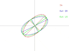
The basic QR algorithm can be visualized in the case where A is a positive-definite symmetric matrix. In that case, A can be depicted as an ellipse in 2 dimensions or an ellipsoid in higher dimensions. The relationship between the input to the algorithm and a single iteration can then be depicted as in Figure 1 (click to see an animation). Note that the LR algorithm is depicted alongside the QR algorithm.

A single iteration causes the ellipse to tilt or "fall" towards the x-axis. In the event where the large semi-axis of the ellipse is parallel to the x-axis, one iteration of QR does nothing. Another situation where the algorithm "does nothing" is when the large semi-axis is parallel to the y-axis instead of the x-axis. In that event, the ellipse can be thought of as balancing precariously without being able to fall in either direction. In both situations, the matrix is diagonal. A situation where an iteration of the algorithm "does nothing" is called a fixed point. The strategy employed by the algorithm is iteration towards a fixed-point. Observe that one fixed point is stable while the other is unstable. If the ellipse were tilted away from the unstable fixed point by a very small amount, one iteration of QR would cause the ellipse to tilt away from the fixed point instead of towards. Eventually though, the algorithm would converge to a different fixed point, but it would take a long time.

Finding eigenvalues versus finding eigenvectors

It's worth pointing out that finding even a single eigenvector of a symmetric matrix is not computable (in exact real arithmetic according to the definitions in computable analysis).^[8] This difficulty exists whenever the multiplicities of a matrix's eigenvalues are not knowable. On the other hand, the same problem does not exist for finding eigenvalues. The eigenvalues of a matrix are always computable.

We will now discuss how these difficulties manifest in the basic QR algorithm. This is illustrated in Figure 2. Recall that the ellipses represent positive-definite symmetric matrices. As the two eigenvalues of the input matrix approach each other, the input ellipse changes into a circle. A circle corresponds to a multiple of the identity matrix. A near-circle corresponds to a near-multiple of the identity matrix whose eigenvalues are nearly equal to the diagonal entries of the matrix. Therefore the problem of approximately finding the eigenvalues is shown to be easy in that case. But notice what happens to the semi-axes of the ellipses. An iteration of QR (or LR) tilts the semi-axes less and less as the input ellipse gets closer to being a circle. The eigenvectors can only be known when the semi-axes are parallel to the x-axis and y-axis. The number of iterations needed to achieve near-parallelism increases without bound as the input ellipse becomes more circular.

While it may be impossible to compute the eigendecomposition of an arbitrary symmetric matrix, it is always possible to perturb the matrix by an arbitrarily small amount and compute the eigendecomposition of the resulting matrix. In the case when the matrix is depicted as a near-circle, the matrix can be replaced with one whose depiction is a perfect circle. In that case, the matrix is a multiple of the identity matrix, and its eigendecomposition is immediate. Be aware though that the resulting eigenbasis can be quite far from the original eigenbasis.

Speeding up: Shifting and deflation

The slowdown when the ellipse gets more circular has a converse: It turns out that when the ellipse gets more stretched - and less circular - then the rotation of the ellipse becomes faster. Such a stretch can be induced when the matrix ${\displaystyle M}$ which the ellipse represents gets replaced with ${\displaystyle M-\lambda I}$ where ${\displaystyle \lambda }$ is approximately the smallest eigenvalue of ${\displaystyle M}$. In this case, the ratio of the two semi-axes of the ellipse approaches ${\displaystyle \infty }$. In higher dimensions, shifting like this makes the length of the smallest semi-axis of an ellipsoid small relative to the other semi-axes, which speeds up convergence to the smallest eigenvalue, but does not speed up convergence to the other eigenvalues. This becomes useless when the smallest eigenvalue is fully determined, so the matrix must then be deflated, which simply means removing its last row and column.

The issue with the unstable fixed point also needs to be addressed. The shifting heuristic is often designed to deal with this problem as well: Practical shifts are often discontinuous and randomised. Wilkinson's shift -- which is well-suited for symmetric matrices like the ones we're visualising -- is in particular discontinuous.

The implicit QR algorithm

In modern computational practice, the QR algorithm is performed in an implicit version which makes the use of multiple shifts easier to introduce.^[4] The matrix is first brought to upper Hessenberg form ${\displaystyle A_{0}=QAQ^{\mathsf {T}}}$ as in the explicit version; then, at each step, the first column of ${\displaystyle A_{k}}$ is transformed via a small-size Householder similarity transformation to the first column of ${\displaystyle p(A_{k})}$^{[clarification needed]} (or ${\displaystyle p(A_{k})e_{1}}$), where ${\displaystyle p(A_{k})}$, of degree ${\displaystyle r}$, is the polynomial that defines the shifting strategy (often ${\displaystyle p(x)=(x-\lambda )(x-{\bar {\lambda }})}$, where ${\displaystyle \lambda }$ and ${\displaystyle {\bar {\lambda }}}$ are the two eigenvalues of the trailing ${\displaystyle 2\times 2}$ principal submatrix of ${\displaystyle A_{k}}$, the so-called implicit double-shift). Then successive Householder transformations of size ${\displaystyle r+1}$ are performed in order to return the working matrix ${\displaystyle A_{k}}$ to upper Hessenberg form. This operation is known as bulge chasing, due to the peculiar shape of the non-zero entries of the matrix along the steps of the algorithm. As in the first version, deflation is performed as soon as one of the sub-diagonal entries of ${\displaystyle A_{k}}$ is sufficiently small.

Renaming proposal

Since in the modern implicit version of the procedure no QR decompositions are explicitly performed, some authors, for instance Watkins,^[9] suggested changing its name to Francis algorithm. Golub and Van Loan use the term Francis QR step.

Interpretation and convergence

The QR algorithm can be seen as a more sophisticated variation of the basic "power" eigenvalue algorithm. Recall that the power algorithm repeatedly multiplies A times a single vector, normalizing after each iteration. The vector converges to an eigenvector of the largest eigenvalue. Instead, the QR algorithm works with a complete basis of vectors, using QR decomposition to renormalize (and orthogonalize). For a symmetric matrix A, upon convergence, AQ = QΛ, where Λ is the diagonal matrix of eigenvalues to which A converged, and where Q is a composite of all the orthogonal similarity transforms required to get there. Thus the columns of Q are the eigenvectors.

History

The QR algorithm was preceded by the LR algorithm, which uses the LU decomposition instead of the QR decomposition. The QR algorithm is more stable, so the LR algorithm is rarely used nowadays. However, it represents an important step in the development of the QR algorithm.

The LR algorithm was developed in the early 1950s by Heinz Rutishauser, who worked at that time as a research assistant of Eduard Stiefel at ETH Zurich. Stiefel suggested that Rutishauser use the sequence of moments y₀^T A^k x₀, k = 0, 1, … (where x₀ and y₀ are arbitrary vectors) to find the eigenvalues of A. Rutishauser took an algorithm of Alexander Aitken for this task and developed it into the quotient–difference algorithm or qd algorithm. After arranging the computation in a suitable shape, he discovered that the qd algorithm is in fact the iteration A_k = L_kU_k (LU decomposition), A_k+1 = U_kL_k, applied on a tridiagonal matrix, from which the LR algorithm follows.^[10]

Other variants

One variant of the QR algorithm, the Golub-Kahan-Reinsch algorithm starts with reducing a general matrix into a bidiagonal one.^[11] This variant of the QR algorithm for the computation of singular values was first described by Golub & Kahan (1965). The LAPACK subroutine DBDSQR implements this iterative method, with some modifications to cover the case where the singular values are very small (Demmel & Kahan 1990). Together with a first step using Householder reflections and, if appropriate, QR decomposition, this forms the DGESVD routine for the computation of the singular value decomposition. The QR algorithm can also be implemented in infinite dimensions with corresponding convergence results.^[12][13]

References

Sources

• Demmel, James; Kahan, William (1990). "Accurate singular values of bidiagonal matrices". SIAM Journal on Scientific and Statistical Computing. 11 (5): 873–912. CiteSeerX 10.1.1.48.3740. doi:10.1137/0911052.
• Golub, Gene H.; Kahan, William (1965). "Calculating the singular values and pseudo-inverse of a matrix". Journal of the Society for Industrial and Applied Mathematics, Series B: Numerical Analysis. 2 (2): 205–224. Bibcode:1965SJNA....2..205G. doi:10.1137/0702016. JSTOR 2949777.

External links

• Eigenvalue problem at PlanetMath.
• Notes on orthogonal bases and the workings of the QR algorithm by Peter J. Olver
• Module for the QR Method
• C++ Library

References

- ^ J.G.F. Francis, "The QR Transformation, I", The Computer Journal, 4(3), pages 265–271 (1961, received October 1959). doi:10.1093/comjnl/4.3.265
- ^ Francis, J. G. F. (1962). "The QR Transformation, II". The Computer Journal. 4 (4): 332–345. doi:10.1093/comjnl/4.4.332.
- ^ Vera N. Kublanovskaya, "On some algorithms for the solution of the complete eigenvalue problem," USSR Computational Mathematics and Mathematical Physics, vol. 1, no. 3, pages 637–657 (1963, received Feb 1961). Also published in: Zhurnal Vychislitel'noi Matematiki i Matematicheskoi Fiziki, vol.1, no. 4, pages 555–570 (1961). doi:10.1016/0041-5553(63)90168-X
- ^ a b Golub, G. H.; Van Loan, C. F. (1996). Matrix Computations (3rd ed.). Baltimore: Johns Hopkins University Press. ISBN 0-8018-5414-8.
- ^ a b Demmel, James W. (1997). Applied Numerical Linear Algebra. SIAM.
- ^ a b Trefethen, Lloyd N.; Bau, David (1997). Numerical Linear Algebra. SIAM.
- ^ Ortega, James M.; Kaiser, Henry F. (1963). "The LLT and QR methods for symmetric tridiagonal matrices". The Computer Journal. 6 (1): 99–101. doi:10.1093/comjnl/6.1.99.
- ^ "linear algebra - Why is uncomputability of the spectral decomposition not a problem?". MathOverflow. Retrieved 2021-08-09.
- ^ Watkins, David S. (2007). The Matrix Eigenvalue Problem: GR and Krylov Subspace Methods. Philadelphia, PA: SIAM. ISBN 978-0-89871-641-2.
- ^ Parlett, Beresford N.; Gutknecht, Martin H. (2011), "From qd to LR, or, how were the qd and LR algorithms discovered?" (PDF), IMA Journal of Numerical Analysis, 31 (3): 741–754, doi:10.1093/imanum/drq003, hdl:20.500.11850/159536, ISSN 0272-4979
- ^ Bochkanov Sergey Anatolyevich. ALGLIB User Guide - General Matrix operations - Singular value decomposition . ALGLIB Project. 2010-12-11. URL:[1] Accessed: 2010-12-11. (Archived by WebCite at https://www.webcitation.org/5utO4iSnR?url=http://www.alglib.net/matrixops/general/svd.php
- ^ Deift, Percy; Li, Luenchau C.; Tomei, Carlos (1985). "Toda flows with infinitely many variables". Journal of Functional Analysis. 64 (3): 358–402. doi:10.1016/0022-1236(85)90065-5.
- ^ Colbrook, Matthew J.; Hansen, Anders C. (2019). "On the infinite-dimensional QR algorithm". Numerische Mathematik. 143 (1): 17–83. arXiv:2011.08172. doi:10.1007/s00211-019-01047-5.