Plug flow reactor model

The plug flow reactor model (PFR, sometimes called continuous tubular reactor, CTR, or piston flow reactors) is a model used to describe chemical reactions in continuous, flowing systems of cylindrical geometry. The PFR model is used to predict the behavior of chemical reactors of such design, so that key reactor variables, such as the dimensions of the reactor, can be estimated.

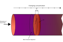
Fluid going through a PFR may be modeled as flowing through the reactor as a series of infinitely thin coherent "plugs", each with a uniform composition, traveling in the axial direction of the reactor, with each plug having a different composition from the ones before and after it. The key assumption is that as a plug flows through a PFR, the fluid is perfectly mixed in the radial direction but not in the axial direction (forwards or backwards). Each plug of differential volume is considered as a separate entity, effectively an infinitesimally small continuous stirred tank reactor, limiting to zero volume. As it flows down the tubular PFR, the residence time (${\displaystyle \tau }$) of the plug is a function of its position in the reactor. In the ideal PFR, the residence time distribution is therefore a Dirac delta function with a value equal to ${\displaystyle \tau }$.

PFR modeling

The stationary PFR is governed by ordinary differential equations, the solution for which can be calculated providing that appropriate boundary conditions are known.

The PFR model works well for many fluids: liquids, gases, and slurries. Although turbulent flow and axial diffusion cause a degree of mixing in the axial direction in real reactors, the PFR model is appropriate when these effects are sufficiently small that they can be ignored.

In the simplest case of a PFR model, several key assumptions must be made in order to simplify the problem, some of which are outlined below. Note that not all of these assumptions are necessary, however the removal of these assumptions does increase the complexity of the problem. The PFR model can be used to model multiple reactions as well as reactions involving changing temperatures, pressures and densities of the flow. Although these complications are ignored in what follows, they are often relevant to industrial processes.

Assumptions:

• Plug flow
• Steady state
• Constant density (reasonable for some liquids but a 20% error for polymerizations; valid for gases only if there is no pressure drop, no net change in the number of moles, nor any large temperature change)
• Single reaction occurring in the bulk of the fluid (homogeneously).

A material balance on the differential volume of a fluid element, or plug, on species i of axial length dx between x and x + dx gives:

[accumulation] = [in] - [out] + [generation] - [consumption]

Accumulation is 0 under steady state; therefore, the above mass balance can be re-written as follows:

1. ${\displaystyle F_{i}(x)-F_{i}(x+dx)+A_{t}dx\nu _{i}r=0}$ .^[1]

where:

• x is the reactor tube axial position, m
• dx the differential thickness of fluid plug
• the index i refers to the species i
• F_i(x) is the molar flow rate of species i at the position x, mol/s
• D is the tube diameter, m
• A_t is the tube transverse cross sectional area, m²
• ν is the stoichiometric coefficient, dimensionless
• r is the volumetric source/sink term (the reaction rate), mol/m³s.

The flow linear velocity, u (m/s) and the concentration of species i, C_i (mol/m³) can be introduced as:

${\displaystyle u={\frac {\dot {v}}{A_{t}}}={\frac {4{\dot {v}}}{\pi D^{2}}}}$ and ${\displaystyle F_{i}=A_{t}uC_{i}\,}$

where ${\displaystyle {\dot {v}}}$ is the volumetric flow rate.

On application of the above to Equation 1, the mass balance on i becomes:

2. ${\displaystyle A_{t}u[C_{i}(x)-C_{i}(x+dx)]+A_{t}dx\nu _{i}r=0\,}$.^[1]

When like terms are cancelled and the limit dx → 0 is applied to Equation 2 the mass balance on species i becomes

3. ${\displaystyle u{\frac {dC_{i}}{dx}}=\nu _{i}r}$,^[1]

The temperature dependence of the reaction rate, r, can be estimated using the Arrhenius equation. Generally, as the temperature increases so does the rate at which the reaction occurs. Residence time, ${\displaystyle \tau }$, is the average amount of time a discrete quantity of reagent spends inside the tank.

Assume:

• isothermal conditions, or constant temperature (k is constant)
• single, irreversible reaction (ν_A = -1)
• first-order reaction (r = k C_A)

After integration of Equation 3 using the above assumptions, solving for C_A(x) we get an explicit equation for the concentration of species A as a function of position:

4. ${\displaystyle C_{A}(x)=C_{A0}e^{-k\tau }\,}$,

where C_A0 is the concentration of species A at the inlet to the reactor, appearing from the integration boundary condition.

Operation and uses

PFRs are used to model the chemical transformation of compounds as they are transported in systems resembling "pipes". The "pipe" can represent a variety of engineered or natural conduits through which liquids or gases flow. (e.g. rivers, pipelines, regions between two mountains, etc.)

An ideal plug flow reactor has a fixed residence time: Any fluid (plug) that enters the reactor at time ${\displaystyle t}$ will exit the reactor at time ${\displaystyle t+\tau }$, where ${\displaystyle \tau }$ is the residence time of the reactor. The residence time distribution function is therefore a Dirac delta function at ${\displaystyle \tau }$. A real plug flow reactor has a residence time distribution that is a narrow pulse around the mean residence time distribution.

A typical plug flow reactor could be a tube packed with some solid material (frequently a catalyst). Typically these types of reactors are called packed bed reactors or PBR's. Sometimes the tube will be a tube in a shell and tube heat exchanger.

When a plug flow model can not be applied, the dispersion model is usually employed.^[2][3]

Residence-time distribution

The residence-time distribution (RTD) of a reactor is a characteristic of the mixing that occurs in the chemical reactor. There is no axial mixing in a plug-flow reactor, and this omission is reflected in the RTD which is exhibited by this class of reactors.^[4]

Real plug flow reactors do not satisfy the idealized flow patterns, back mix flow or plug flow deviation from ideal behavior can be due to channeling of fluid through the vessel, recycling of fluid within the vessel or due to the presence of stagnant region or dead zone of fluid in the vessel.^[5] Real plug flow reactors with non-ideal behavior have also been modelled.^[6] To predict the exact behavior of a vessel as a chemical reactor, RTD or stimulus response technique is used. The tracer technique, the most widely used method for the study of axial dispersion, is usually used in the form of:^[7]

• Pulse input
• Step input
• Cyclic input
• Random input

The RTD is determined experimentally by injecting an inert chemical, molecule, or atom, called a tracer, into the reactor at some time t = 0 and then measuring the tracer concentration, C, in the effluent stream as a function of time.^[4]

The RTD curve of fluid leaving a vessel is called the E-Curve. This curve is normalized in such a way that the area under it is unity:

(1)

${\displaystyle \int E\partial t=1}$

The mean age of the exit stream or mean residence time is:

(2)

${\displaystyle \tau =\int tE\partial t=\sum tE\nabla t}$

When a tracer is injected into a reactor at a location more than two or three particle diameters downstream from the entrance and measured some distance upstream from the exit, the system can be described by the dispersion model with combinations of open or close boundary conditions.^[3] For such a system where there is no discontinuity in type of flow at the point of tracer injection or at the point of tracer measurement, the variance for open-open system is:

(3)

${\displaystyle (\sigma _{\theta })^{2}=(\sigma _{t})^{2}/\tau ^{2}=2/P_{e}+8/(P_{e})^{2}}$

Where,

(4)

${\displaystyle P_{e}=LU/D_{L}}$

which represents the ratio of rate of transport by convection to rate of transport by diffusion or dispersion.

${\displaystyle L}$ = characteristic length (m)

${\displaystyle D_{L}}$ = effective dispersion coefficient ( m²/s)

${\displaystyle U}$ = superficial velocity (m/s) based on empty cross-section

Vessel dispersion number is defined as:

${\displaystyle 1/P_{e}=D_{L}/LU}$

The variance of a continuous distribution measured at a finite number of equidistant locations is given by:

(5)

${\displaystyle (\sigma _{t})^{2}=\sum t_{i}^{2}C_{i}/\sum C_{i}-\sum [t_{i}C_{i}/\sum C_{i}]^{2}}$

Where mean residence time τ is given by:

(6)

${\displaystyle \tau =\sum t_{i}C_{i}/\sum C_{i}}$

(7)

${\displaystyle (\sigma _{\theta })^{2}=(\sigma _{t})^{2}/\tau ^{2}}$

Thus (σ_θ)² can be evaluated from the experimental data on C vs. t and for known values of ${\displaystyle (\sigma _{\theta })^{2}}$, the dispersion number ${\displaystyle (1/P_{e})}$ can be obtained from eq. (3) as:

(8)

${\displaystyle D_{L}/LU={-1+{\sqrt {1+8(\sigma _{\theta })^{2}}} \over 8}}$

Thus axial dispersion coefficient D_L can be estimated (L = packed height)^[5]

As mentioned before, there are also other boundary conditions that can be applied to the dispersion model giving different relationships for the dispersion number.^[8][9][3]

Advantages

From the safety technical point of view the PFTR has the advantages that ^[10]

1. It operates in a steady state
2. It is well controllable
3. Large heat transfer areas can be installed

Concerns

The main problems lies in difficult and sometimes critical start-up and shut down operations.^[10]

Applications

Plug flow reactors are used for some of the following applications:

• Large-scale production
• Fast reactions
• Homogeneous or heterogeneous reactions
• Continuous production
• High-temperature reactions

See also

Reference and sources

This page was last edited on 11 April 2024, at 03:25