Parabolic cylindrical coordinates

In mathematics, parabolic cylindrical coordinates are a three-dimensional orthogonal coordinate system that results from projecting the two-dimensional parabolic coordinate system in the perpendicular $z$ -direction. Hence, the coordinate surfaces are confocal parabolic cylinders. Parabolic cylindrical coordinates have found many applications, e.g., the potential theory of edges.

YouTube Encyclopedic

1/5
Views:
38 904
54 674
8 234
11 750
4 963

Transcription

Three dimensional coordinate systems level three. in the previous video we started to describe basic equations in R cubed. Specifically describing equations on a three-dimensional Cartesian coordinate system in this video we will continue describing basic equations in three-dimensional space. Let's start by graphing the equation y = x in R-squared. Since this graph will provide us with a starting point to successfully graph it in R-cubed. For starters, this equation is represented by a line in R squared and has the form y = mx + b where the slope is equal to one and the y-intercept is equal to zero. So we typically graph these equations by first plotting the y-intercept in this case it's equal to zero, then we use the slope which in this case is equal to one, to generate a second point. recall that a slope of positive one means that we move in the positive y direction one unit and move in the positive x-direction one unit. Remember the slope can be interpreted as the rise over the run. Once we have our two points we go ahead and connect them obtaining the following straight curved. Now if we were to graph this equation in R-cubed we would obtain the same curve in the xy-plane this curve has a y-intercept of zero and a slope of positive one, but notice that the variable z is not mentioned in the equation meaning we have not specified z in any way so we must assume that z can take on any value this means that any particular value of z will get a copy of this line both the positive values of z such as z = 1 z = 2, z = 3, and so on and negative values of z such as z = -1, z = -2, and z = -3 and so on. In this sense the graph represents a vertical plane that lies over the line given by the equation y = x in the xy-plane. Notice that we started by drawing the curve on the plane that contained the variables for which the equation was defined in this case the equation was defined but the variables x and y so we first graphed it on the XY plane, then we drew copies of this curve on both the positive and negative direction of the missing variable which was not expressed in the equation in this case the variable that was not expressed was z remember variable that are not explicitly expressed in the equation are assumed to attain any value unless mentioned otherwise. we will go over equations in which the variables are restricted in a later video. Alright, lets spice things up a bit and graph the equation z = -2y + 1. once again, this equation has the form y = mx + b, but instead we have the equation z = my + b, where z is the dependent variable and y is the independent variable, we essentially treat the equation just like we did in the previous example, but instead of graphing it in the xy-plane we are actually going to graph the curve on the yz-plane as follows, here we have a two-dimensional representation of the yz-plane we're going to graph the curve in this plane and then translate it into R-cubed, so let's go ahead and plot what used to be the y-intercept which in this case is now the z-intercept on the yz-plane so we plot the first points at z = 1, then we use the slope, in this case its negative two, which can be interpreted as negative two over one or in this case the rise over run and use it to generate a second point, so from the z-intercept we go ahead and move two units down along the negative z-axis and move one unit to the right along the positive y-axis then we connect the points with a curve as follows alright, having graphed the equation in the yz-plane we're ready to translate it into the yz-plane of a three-dimensional Cartesian coordinate system its the same idea, but now we need to be able to navigate along the yz-plane of this three-dimensional coordinate system the yz-plane is located here, the positive y-axis is located here and the positive z-axis is here, so we literally draw the same curve we just graphed in R-squared onto the yz-plane of R-cubed as follows next we notice the variable x is not expressed in the equation and there are also no restrictions this means that x can take on any value as a consequence, at any particular value of x there will be a copy of this line both on the positive values of x such as x = 1, x = 2, and x = 3, and so on, and the negative values of x such as x = -1, x = -2, x = -3, and so on, in this sense the graph represents a plane that intercepts the z-axis at z = 1 and has a negative slope the plane is inclined with a slope of negative two over one alright, lets try the next example. This one requires graphing an equation on the xz-plane. Let's graph the equation 2z + 1 = 3x, notice that this equation is not in slope intercept form so we first need to arrange the equation into the slope intercept form of a line, notice that all the concepts you learned in your previous math classes come back in some shape way or form this will be true as we dive deeper into multivariable calculus okay, in order to write the equation in slope intercept form we first need to solve for the dependent variable in this case the dependent variable is z and the independent variable is x this is similar to the way we solved for y when dealing with an equation in the xy-plane back in your pre-calculus class so we go ahead and subtract one from both sides then we divide both sides by two, doing that we obtain the equation z equals three half x minus one half. let's go ahead and graph this equation directly into the three-dimensional coordinate system you first need to graph the curve on the xz-plane so looking at the equation we see that the z-intercept is negative one half so we first plot this point as follows then we noticed that the slope is positive three halves so we use this slope to generate an additional point, so starting from the z-intercept we move three units towards the positive z-axis and two units towards the positive x-axis, then we go ahead and connect a curve connecting both points as follows. Having created our first curve we go ahead and make copies of this curve at positive values of y and at negative values of y, remember when a variable is not expressed in an equation and no restrictions are mentioned the variable is free to take on any value lastly, we connect all the curves together and obtain the following plane that has a z-intercept of negative one half and is also inclined with a slope of positive three halves alright, these three examples were designed to illustrate the fact that you can use all your knowledge and experience from graphing equations in a two-dimensional coordinate system and translate them into three dimensions it might take you some time to get used to but like in all your math classes practice is key in developing this skill. In a later video we will actually develop a more powerful way of describing planes in 3D space. For now, these examples were designed so you can start obtaining an idea of how to navigate through this three-dimensional coordinate system alright, lets try graphing something other than planes let's give it a shot and graph the following equation. x squared plus y squared equals four. Notice that the variables that are explicitly expressed are the variables x and y. so we are going to first graph this equation in R squared specifically on the xy-plane. Recall from your studies of precalculus that this equation represents a circle centered at the origin with radius two, so its graph is represented in R-squared as follows. Now if we want to graph this equation in R-cubed we go ahead and graph this curve on the xy-plane as follows. next we notice that the variable z is not expressed in the equation remember this means that every single value of z both positive and negative will have copies of this curve which has the shape of a circle finally we connect the curves with rulings as follows this equation represents a cylinder centered in the z-axis so in R-squared the equation represents a circle and in R-cubed it represents a cylinder once again this example illustrates the importance of specifying what coordinate system we are referring to, since it ultimately determines the graph the equation aright, let's end the video by graphing one final equation lets graph the equation z equals x squared notice that the variables z and x are expressed in this equation so we're going to go ahead and graph them on the xz-plane in addition, notice that this equation looks like the equation of a parabola of the form y equals x squared but in this case the dependent variable is z and the independent variable is x other than the variable z, this equation pretty much represents a parabola in the xz-plane and is graphed as follows this is how this equation will look like in R-squared next we go ahead and graph the same curve on the xz-plane of R-cubed as follows notice that the variable that is not expressed is y this means that every single value of y will have a copy of this curve since its free to take any value of y, in addition no restrictions have been imposed on the variable y. Next we go ahead and connect the curves as follows, doing that we obtain the following surface this surface is called a parabolic cylinder we will study this surface and many more in a later video for now, keep in mind that equations in R-squared are usually represented by curves on a plane and equations in R-cubed are usually represented by a surface but not always they can also be represented by curves in space as we will see in a later video. Alright in our next video we will start exploring common formulas associated with a three-dimensional coordinate system

Basic definition

The parabolic cylindrical coordinates $(σ, τ, z)$ are defined in terms of the Cartesian coordinates $(x, y, z)$ by:

{\begin{aligned}x&=\sigma \tau \\y&={\frac {1}{2}}\left(\tau ^{2}-\sigma ^{2}\right)\\z&=z\end{aligned}}

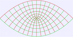
The surfaces of constant $σ$ form confocal parabolic cylinders

2y={\frac {x^{2}}{\sigma ^{2}}}-\sigma ^{2}

that open towards $+ y$ , whereas the surfaces of constant $τ$ form confocal parabolic cylinders

2y=-{\frac {x^{2}}{\tau ^{2}}}+\tau ^{2}

that open in the opposite direction, i.e., towards $- y$ . The foci of all these parabolic cylinders are located along the line defined by $x = y = 0$ . The radius $r$ has a simple formula as well

r={\sqrt {x^{2}+y^{2}}}={\frac {1}{2}}\left(\sigma ^{2}+\tau ^{2}\right)

that proves useful in solving the Hamilton–Jacobi equation in parabolic coordinates for the inverse-square central force problem of mechanics; for further details, see the Laplace–Runge–Lenz vector article.

Scale factors

The scale factors for the parabolic cylindrical coordinates $σ$ and $τ$ are:

{\begin{aligned}h_{\sigma }&=h_{\tau }={\sqrt {\sigma ^{2}+\tau ^{2}}}\\h_{z}&=1\end{aligned}}

Differential elements

The infinitesimal element of volume is

dV=h_{\sigma }h_{\tau }h_{z}d\sigma d\tau dz=(\sigma ^{2}+\tau ^{2})d\sigma \,d\tau \,dz

The differential displacement is given by:

d\mathbf {l} ={\sqrt {\sigma ^{2}+\tau ^{2}}}\,d\sigma \,{\boldsymbol {\hat {\sigma }}}+{\sqrt {\sigma ^{2}+\tau ^{2}}}\,d\tau \,{\boldsymbol {\hat {\tau }}}+dz\,\mathbf {\hat {z}}

The differential normal area is given by:

d\mathbf {S} ={\sqrt {\sigma ^{2}+\tau ^{2}}}\,d\tau \,dz{\boldsymbol {\hat {\sigma }}}+{\sqrt {\sigma ^{2}+\tau ^{2}}}\,d\sigma \,dz{\boldsymbol {\hat {\tau }}}+\left(\sigma ^{2}+\tau ^{2}\right)\,d\sigma \,d\tau \mathbf {\hat {z}}

Del

Let $f$ be a scalar field. The gradient is given by

\nabla f={\frac {1}{\sqrt {\sigma ^{2}+\tau ^{2}}}}{\partial f \over \partial \sigma }{\boldsymbol {\hat {\sigma }}}+{\frac {1}{\sqrt {\sigma ^{2}+\tau ^{2}}}}{\partial f \over \partial \tau }{\boldsymbol {\hat {\tau }}}+{\partial f \over \partial z}\mathbf {\hat {z}}

The Laplacian is given by

\nabla ^{2}f={\frac {1}{\sigma ^{2}+\tau ^{2}}}\left({\frac {\partial ^{2}f}{\partial \sigma ^{2}}}+{\frac {\partial ^{2}f}{\partial \tau ^{2}}}\right)+{\frac {\partial ^{2}f}{\partial z^{2}}}

Let $A$ be a vector field of the form:

\mathbf {A} =A_{\sigma }{\boldsymbol {\hat {\sigma }}}+A_{\tau }{\boldsymbol {\hat {\tau }}}+A_{z}\mathbf {\hat {z}}

The divergence is given by

\nabla \cdot \mathbf {A} ={\frac {1}{\sigma ^{2}+\tau ^{2}}}\left({\partial ({\sqrt {\sigma ^{2}+\tau ^{2}}}A_{\sigma }) \over \partial \sigma }+{\partial ({\sqrt {\sigma ^{2}+\tau ^{2}}}A_{\tau }) \over \partial \tau }\right)+{\partial A_{z} \over \partial z}

The curl is given by

\nabla \times \mathbf {A} =\left({\frac {1}{\sqrt {\sigma ^{2}+\tau ^{2}}}}{\frac {\partial A_{z}}{\partial \tau }}-{\frac {\partial A_{\tau }}{\partial z}}\right){\boldsymbol {\hat {\sigma }}}-\left({\frac {1}{\sqrt {\sigma ^{2}+\tau ^{2}}}}{\frac {\partial A_{z}}{\partial \sigma }}-{\frac {\partial A_{\sigma }}{\partial z}}\right){\boldsymbol {\hat {\tau }}}+{\frac {1}{\sigma ^{2}+\tau ^{2}}}\left({\frac {\partial \left({\sqrt {\sigma ^{2}+\tau ^{2}}}A_{\tau }\right)}{\partial \sigma }}-{\frac {\partial \left({\sqrt {\sigma ^{2}+\tau ^{2}}}A_{\sigma }\right)}{\partial \tau }}\right)\mathbf {\hat {z}}

Other differential operators can be expressed in the coordinates $(σ, τ)$ by substituting the scale factors into the general formulae found in orthogonal coordinates.

Relationship to other coordinate systems

Relationship to cylindrical coordinates $(ρ, φ, z)$ :

{\begin{aligned}\rho \cos \varphi &=\sigma \tau \\\rho \sin \varphi &={\frac {1}{2}}\left(\tau ^{2}-\sigma ^{2}\right)\\z&=z\end{aligned}}

Parabolic unit vectors expressed in terms of Cartesian unit vectors:

{\begin{aligned}{\boldsymbol {\hat {\sigma }}}&={\frac {\tau {\hat {\mathbf {x} }}-\sigma {\hat {\mathbf {y} }}}{\sqrt {\tau ^{2}+\sigma ^{2}}}}\\{\boldsymbol {\hat {\tau }}}&={\frac {\sigma {\hat {\mathbf {x} }}+\tau {\hat {\mathbf {y} }}}{\sqrt {\tau ^{2}+\sigma ^{2}}}}\\\mathbf {\hat {z}} &=\mathbf {\hat {z}} \end{aligned}}

Parabolic cylinder harmonics

Since all of the surfaces of constant $σ$ , $τ$ and $z$ are conicoids, Laplace's equation is separable in parabolic cylindrical coordinates. Using the technique of the separation of variables, a separated solution to Laplace's equation may be written:

V=S(\sigma )T(\tau )Z(z)

and Laplace's equation, divided by $V$ , is written:

{\frac {1}{\sigma ^{2}+\tau ^{2}}}\left[{\frac {\ddot {S}}{S}}+{\frac {\ddot {T}}{T}}\right]+{\frac {\ddot {Z}}{Z}}=0

Since the $Z$ equation is separate from the rest, we may write

{\frac {\ddot {Z}}{Z}}=-m^{2}

where $m$ is constant. $Z (z)$ has the solution:

Z_{m}(z)=A_{1}\,e^{imz}+A_{2}\,e^{-imz}

Substituting $- m 2$ for ${\ddot {Z}}/Z$ , Laplace's equation may now be written:

\left[{\frac {\ddot {S}}{S}}+{\frac {\ddot {T}}{T}}\right]=m^{2}(\sigma ^{2}+\tau ^{2})

We may now separate the $S$ and $T$ functions and introduce another constant $n 2$ to obtain:

{\ddot {S}}-(m^{2}\sigma ^{2}+n^{2})S=0

{\ddot {T}}-(m^{2}\tau ^{2}-n^{2})T=0

The solutions to these equations are the parabolic cylinder functions

S_{mn}(\sigma )=A_{3}y_{1}(n^{2}/2m,\sigma {\sqrt {2m}})+A_{4}y_{2}(n^{2}/2m,\sigma {\sqrt {2m}})

T_{mn}(\tau )=A_{5}y_{1}(n^{2}/2m,i\tau {\sqrt {2m}})+A_{6}y_{2}(n^{2}/2m,i\tau {\sqrt {2m}})

The parabolic cylinder harmonics for $(m, n)$ are now the product of the solutions. The combination will reduce the number of constants and the general solution to Laplace's equation may be written:

V(\sigma ,\tau ,z)=\sum _{m,n}A_{mn}S_{mn}T_{mn}Z_{m}

Applications

The classic applications of parabolic cylindrical coordinates are in solving partial differential equations, e.g., Laplace's equation or the Helmholtz equation, for which such coordinates allow a separation of variables. A typical example would be the electric field surrounding a flat semi-infinite conducting plate.

Bibliography

Morse PM, Feshbach H (1953). Methods of Theoretical Physics, Part I. New York: McGraw-Hill. p. 658. ISBN 0-07-043316-X. LCCN 52011515.
Margenau H, Murphy GM (1956). The Mathematics of Physics and Chemistry. New York: D. van Nostrand. pp. 186–187. LCCN 55010911.
Korn GA, Korn TM (1961). Mathematical Handbook for Scientists and Engineers. New York: McGraw-Hill. p. 181. LCCN 59014456. ASIN B0000CKZX7.
Sauer R, Szabó I (1967). Mathematische Hilfsmittel des Ingenieurs. New York: Springer Verlag. p. 96. LCCN 67025285.
Zwillinger D (1992). Handbook of Integration. Boston, MA: Jones and Bartlett. p. 114. ISBN 0-86720-293-9. Same as Morse & Feshbach (1953), substituting u_k for ξ_k.
Moon P, Spencer DE (1988). "Parabolic-Cylinder Coordinates (μ, ν, z)". Field Theory Handbook, Including Coordinate Systems, Differential Equations, and Their Solutions (corrected 2nd ed., 3rd print ed.). New York: Springer-Verlag. pp. 21–24 (Table 1.04). ISBN 978-0-387-18430-2.

External links

MathWorld description of parabolic cylindrical coordinates

v t e Orthogonal coordinate systems
Two dimensional	Cartesian Polar (Log-polar) Parabolic Bipolar Elliptic
Three dimensional	Cartesian Cylindrical Spherical Parabolic Paraboloidal Oblate spheroidal Prolate spheroidal Ellipsoidal Elliptic cylindrical Toroidal Bispherical Bipolar cylindrical Conical 6-sphere

This page was last edited on 7 August 2022, at 14:32

From Wikipedia, the free encyclopedia