
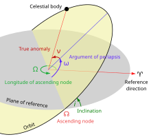
In celestial mechanics, the longitude of the periapsis, also called longitude of the pericenter, of an orbiting body is the longitude (measured from the point of the vernal equinox) at which the periapsis (closest approach to the central body) would occur if the body's orbit inclination were zero. It is usually denoted ϖ.
For the motion of a planet around the Sun, this position is called longitude of perihelion ϖ, which is the sum of the longitude of the ascending node Ω, and the argument of perihelion ω.[1][2]
The longitude of periapsis is a compound angle, with part of it being measured in the plane of reference and the rest being measured in the plane of the orbit. Likewise, any angle derived from the longitude of periapsis (e.g., mean longitude and true longitude) will also be compound.
Sometimes, the term longitude of periapsis is used to refer to ω, the angle between the ascending node and the periapsis. That usage of the term is especially common in discussions of binary stars and exoplanets.[3][4] However, the angle ω is less ambiguously known as the argument of periapsis.
YouTube Encyclopedic
-
1/3Views:24 0806 2674 024
-
Satellite Orbit Analysis and Simulation (in MATLAB)
-
Teach Astronomy - Perihelion and Aphelion
-
# Keplerian Elements : Orbital Inclination and the Right Ascension of Ascending Node (RAAN)
Transcription
OK guys, today I'm gonna show you a little software I made. It's an orbit analysis software and what it does is it's basically gonna input a position vector in kilometers of a satellite and its velocity direction vector and its magnitude and what it's gonna show you is it's orbit in 3D space around the Earth. Taking in to consideration the simple gravity and no other objects will be taken into consideration, no moon, just a simple satellite around Earth orbit and as you can see we have a few more parameters here - just a little runspeed because some orbits are extremely long and some orbits are shorter and just to fit it in to a good time we have a little runspeed right here. We have a rev number which is the number of revolutions I want it to perform and a really interesting thing right here called the number of days J2000 which is the number of days since January 1st, 2000 and what that does is it's going to line up a little picture of the Earth exactly at the time frame you want it, so if you have, if it's x hours since 2000, it's gonna line it up right then, I mean, if you want it enter the number of hours as it is right now then its gonna show you the position of the Earth right now. Now, first of all, I'm gonna go ahead and run for you a simple orbit around the Earth - as you can see 7000, 0 , 0 at a velocity of 7500 m/s. Oh, let's run this. Oh and after it runs, it's gonna plot out the ground track of the satellite which is essentially a track on the Earth of what the satellite can see directly above when it's orbitting the Earth. Here we go. Okay, you can see it's a very low Earth orbit, it's revolving really fast. It's going around the green little thing is the initial position and the green line denotes the.. that's the ground track right here. Let it run - let it finish running. Okay let's go back here. Now, as you can see that little green thing denotes the initial position of the satellite, and the green line represents the velocity vector initially. You can turn this figure around. That red line is where the revolution of the satellite just ended. You can see a picture representation of the Earth. We have these two sets of axeses if you can see them clear and further examples, but what these examples denote. Well the black ones denote a fixed inertial frame, and the red ones that revolve around along with the Earth. I'm sorry, I'm sorry. The red ones a re a fixed frame and the black ones revolve along with the Earth, and for this little simple orbit right here we have a ground track really similar to a sine wave right here and well, that's essentially it - looks simple enough, doesn't it? Let's go check out some cooler orbits. We're gonna check out a geostationary orbit. As you can see we have all the values saved right here. Vmag, 2072, we'll put it at a runspeed of a 1000 because it's very far away from the Earth and a geostationary orbit as you can see here, is always focussed over one particular position on the ground on the Earth's surface. And let it complete that 5th revolution and as you can see that ground track really isn't changing. The program's still running, mind you, but the ground track remains this little small red dot, which happens to be off the coast of Australia and well, that's one orbit - that's called a Geostationary orbit. I'm gonna show you one more before we're done here and it's called a Molniya orbit, and what's cool about a Molniya orbit is its ground track , it's a really funny ground track - it's not exactly sinusoidal but it's not a fixed point like the Geostationary one, well let me surprise you.. Here we go, let me run this one more time. As you can see, it's a very elliptical orbit this one. The satellite goes really far away - you can see that yellow line decreasing and increasing. Mind you, the speed is exactly the speed the satellite would rotate in real time Earth and it follows all of Kepler's laws. And if you see right here if we rotate it in a different direction - let it complete that 5th revolution right here. You can even zoom in if you wanted to. Let it revolve. And yeah, you can see the ground track of a Molniya orbit - it goes up and stays there for a while and suddenly swishes back down to form this little lasso kind of shape I guess. And i guess, that's what's cool about it, I mean, it's a little lasso shaped, it's not sinusoidal. I'm gonna wait for it to finish all its little lassos. You can see this really nice representation of the Earth in 2D - you can do that intrinsically through a little MATLAB function and you see it goes really slow on the edges of the lasso and that's because when it's coming down it's closer to the Earth and it's revolving at a quicker speed and when it's further away, it's slow, and the Earth's rotation is what makes up.. it's what causes the movement essentially - I dunno how better to put it. And one more.. See it's really slowing down right here. Go back to this - this really cool visualization. And that's it guys - that's my orbit analysis software. You can ask any questions about how I did this. Feel free. It's my first video on YouTube. Please subscribe, and please comment and like this video. Thank you.
Calculation from state vectors
ϖ is the sum of the longitude of ascending node Ω (measured on ecliptic plane) and the argument of periapsis ω (measured on orbital plane):

which are derived from the orbital state vectors.
Derivation of ecliptic longitude and latitude of perihelion for inclined orbits
Define the following:
- i, inclination
- ω, argument of perihelion
- Ω, longitude of ascending node
- ε, obliquity of the ecliptic (for the standard equinox of 2000.0, use 23.43929111°)
Then:
- A = cos ω cos Ω – sin ω sin Ω cos i
- B = cos ε (cos ω sin Ω + sin ω cos Ω cos i) – sin ε sin ω sin i
- C = sin ε (cos ω sin Ω + sin ω cos Ω cos i) + cos ε sin ω sin i
The right ascension α and declination δ of the direction of perihelion are:
If A < 0, add 180° to α to obtain the correct quadrant.
The ecliptic longitude ϖ and latitude b of perihelion are:
If cos(α) < 0, add 180° to ϖ to obtain the correct quadrant.
As an example, using the most up-to-date numbers from Brown (2017)[5] for the hypothetical Planet Nine with i = 30°, ω = 136.92°, and Ω = 94°, then α = 237.38°, δ = +0.41° and ϖ = 235.00°, b = +19.97° (Brown actually provides i, Ω, and ϖ, from which ω was computed).
References
- ^ Urban, Sean E.; Seidelmann, P. Kenneth (eds.). "Chapter 8: Orbital Ephemerides of the Sun, Moon, and Planets" (PDF). Explanatory Supplement to the Astronomical Almanac. University Science Books. p. 26.
- ^ Simon, J. L.; et al. (1994). "Numerical expressions for precession formulae and mean elements for the Moon and the planets". Astronomy and Astrophysics. 282: 663–683, 672. Bibcode:1994A&A...282..663S.
- ^ Robert Grant Aitken (1918). The Binary Stars. Semicentennial Publications of the University of California. D.C. McMurtrie. p. 201.
- ^ "Format" Archived 2009-02-25 at the Wayback Machine in Sixth Catalog of Orbits of Visual Binary Stars Archived 2009-04-12 at the Wayback Machine, William I. Hartkopf & Brian D. Mason, U.S. Naval Observatory, Washington, D.C. Accessed on 10 January 2018.
- ^ Brown, Michael E. (2017) “Planet Nine: where are you? (part 1)” The Search for Planet Nine. http://www.findplanetnine.com/2017/09/planet-nine-where-are-you-part-1.html
External links
- Determination of the Earth's Orbital Parameters Past and future longitude of perihelion for Earth.
Gravitational orbits | |||||||||
|---|---|---|---|---|---|---|---|---|---|
| Types |
| ||||||||
| Parameters |
| ||||||||
| Maneuvers | |||||||||
| Orbital mechanics |
| ||||||||