Linearization

In mathematics, linearization is finding the linear approximation to a function at a given point. The linear approximation of a function is the first order Taylor expansion around the point of interest. In the study of dynamical systems, linearization is a method for assessing the local stability of an equilibrium point of a system of nonlinear differential equations or discrete dynamical systems.^[1] This method is used in fields such as engineering, physics, economics, and ecology.

Linearization of a function

Linearizations of a function are lines—usually lines that can be used for purposes of calculation. Linearization is an effective method for approximating the output of a function ${\displaystyle y=f(x)}$ at any ${\displaystyle x=a}$ based on the value and slope of the function at ${\displaystyle x=b}$, given that ${\displaystyle f(x)}$ is differentiable on ${\displaystyle [a,b]}$ (or ${\displaystyle [b,a]}$) and that ${\displaystyle a}$ is close to ${\displaystyle b}$. In short, linearization approximates the output of a function near ${\displaystyle x=a}$.

For example, ${\displaystyle {\sqrt {4}}=2}$. However, what would be a good approximation of ${\displaystyle {\sqrt {4.001}}={\sqrt {4+.001}}}$?

For any given function ${\displaystyle y=f(x)}$, ${\displaystyle f(x)}$ can be approximated if it is near a known differentiable point. The most basic requisite is that ${\displaystyle L_{a}(a)=f(a)}$, where ${\displaystyle L_{a}(x)}$ is the linearization of ${\displaystyle f(x)}$ at ${\displaystyle x=a}$. The point-slope form of an equation forms an equation of a line, given a point ${\displaystyle (H,K)}$ and slope ${\displaystyle M}$. The general form of this equation is: ${\displaystyle y-K=M(x-H)}$.

Using the point ${\displaystyle (a,f(a))}$, ${\displaystyle L_{a}(x)}$ becomes ${\displaystyle y=f(a)+M(x-a)}$. Because differentiable functions are locally linear, the best slope to substitute in would be the slope of the line tangent to ${\displaystyle f(x)}$ at ${\displaystyle x=a}$.

While the concept of local linearity applies the most to points arbitrarily close to ${\displaystyle x=a}$, those relatively close work relatively well for linear approximations. The slope ${\displaystyle M}$ should be, most accurately, the slope of the tangent line at ${\displaystyle x=a}$.

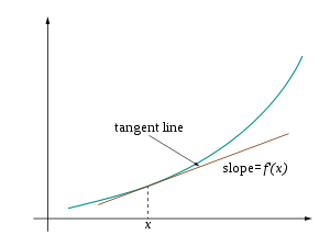
Visually, the accompanying diagram shows the tangent line of ${\displaystyle f(x)}$ at ${\displaystyle x}$. At ${\displaystyle f(x+h)}$, where ${\displaystyle h}$ is any small positive or negative value, ${\displaystyle f(x+h)}$ is very nearly the value of the tangent line at the point ${\displaystyle (x+h,L(x+h))}$.

The final equation for the linearization of a function at ${\displaystyle x=a}$ is:

$${\displaystyle y=(f(a)+f'(a)(x-a))}$$

For ${\displaystyle x=a}$, ${\displaystyle f(a)=f(x)}$. The derivative of ${\displaystyle f(x)}$ is ${\displaystyle f'(x)}$, and the slope of ${\displaystyle f(x)}$ at ${\displaystyle a}$ is ${\displaystyle f'(a)}$.

Example

To find ${\displaystyle {\sqrt {4.001}}}$, we can use the fact that ${\displaystyle {\sqrt {4}}=2}$. The linearization of ${\displaystyle f(x)={\sqrt {x}}}$ at ${\displaystyle x=a}$ is ${\displaystyle y={\sqrt {a}}+{\frac {1}{2{\sqrt {a}}}}(x-a)}$, because the function ${\displaystyle f'(x)={\frac {1}{2{\sqrt {x}}}}}$ defines the slope of the function ${\displaystyle f(x)={\sqrt {x}}}$ at ${\displaystyle x}$. Substituting in ${\displaystyle a=4}$, the linearization at 4 is ${\displaystyle y=2+{\frac {x-4}{4}}}$. In this case ${\displaystyle x=4.001}$, so ${\displaystyle {\sqrt {4.001}}}$ is approximately ${\displaystyle 2+{\frac {4.001-4}{4}}=2.00025}$. The true value is close to 2.00024998, so the linearization approximation has a relative error of less than 1 millionth of a percent.

Linearization of a multivariable function

The equation for the linearization of a function ${\displaystyle f(x,y)}$ at a point ${\displaystyle p(a,b)}$ is:

${\displaystyle f(x,y)\approx f(a,b)+\left.{\frac {\partial f(x,y)}{\partial x}}\right|_{a,b}(x-a)+\left.{\frac {\partial f(x,y)}{\partial y}}\right|_{a,b}(y-b)}$

The general equation for the linearization of a multivariable function ${\displaystyle f(\mathbf {x} )}$ at a point ${\displaystyle \mathbf {p} }$ is:

${\displaystyle f({\mathbf {x} })\approx f({\mathbf {p} })+\left.{\nabla f}\right|_{\mathbf {p} }\cdot ({\mathbf {x} }-{\mathbf {p} })}$

where ${\displaystyle \mathbf {x} }$ is the vector of variables, ${\displaystyle {\nabla f}}$ is the gradient, and ${\displaystyle \mathbf {p} }$ is the linearization point of interest .^[2]

Uses of linearization

Linearization makes it possible to use tools for studying linear systems to analyze the behavior of a nonlinear function near a given point. The linearization of a function is the first order term of its Taylor expansion around the point of interest. For a system defined by the equation

${\displaystyle {\frac {d\mathbf {x} }{dt}}=\mathbf {F} (\mathbf {x} ,t)}$,

the linearized system can be written as

${\displaystyle {\frac {d\mathbf {x} }{dt}}\approx \mathbf {F} (\mathbf {x_{0}} ,t)+D\mathbf {F} (\mathbf {x_{0}} ,t)\cdot (\mathbf {x} -\mathbf {x_{0}} )}$

where ${\displaystyle \mathbf {x_{0}} }$ is the point of interest and ${\displaystyle D\mathbf {F} (\mathbf {x_{0}} ,t)}$ is the ${\displaystyle \mathbf {x} }$-Jacobian of ${\displaystyle \mathbf {F} (\mathbf {x} ,t)}$ evaluated at ${\displaystyle \mathbf {x_{0}} }$.

Stability analysis

In stability analysis of autonomous systems, one can use the eigenvalues of the Jacobian matrix evaluated at a hyperbolic equilibrium point to determine the nature of that equilibrium. This is the content of the linearization theorem. For time-varying systems, the linearization requires additional justification.^[3]

Microeconomics

In microeconomics, decision rules may be approximated under the state-space approach to linearization.^[4] Under this approach, the Euler equations of the utility maximization problem are linearized around the stationary steady state.^[4] A unique solution to the resulting system of dynamic equations then is found.^[4]

Optimization

In mathematical optimization, cost functions and non-linear components within can be linearized in order to apply a linear solving method such as the Simplex algorithm. The optimized result is reached much more efficiently and is deterministic as a global optimum.

Multiphysics

In multiphysics systems—systems involving multiple physical fields that interact with one another—linearization with respect to each of the physical fields may be performed. This linearization of the system with respect to each of the fields results in a linearized monolithic equation system that can be solved using monolithic iterative solution procedures such as the Newton–Raphson method. Examples of this include MRI scanner systems which results in a system of electromagnetic, mechanical and acoustic fields.^[5]

See also

• Linear stability
• Tangent stiffness matrix
• Stability derivatives
• Linearization theorem
• Taylor approximation
• Functional equation (L-function)

References

External links

Linearization tutorials

• Linearization for Model Analysis and Control Design

This page was last edited on 9 June 2023, at 02:39

References

- ^ The linearization problem in complex dimension one dynamical systems at Scholarpedia
- ^ Linearization. The Johns Hopkins University. Department of Electrical and Computer Engineering Archived 2010-06-07 at the Wayback Machine
- ^ Leonov, G. A.; Kuznetsov, N. V. (2007). "Time-Varying Linearization and the Perron effects". International Journal of Bifurcation and Chaos. 17 (4): 1079–1107. Bibcode:2007IJBC...17.1079L. doi:10.1142/S0218127407017732.
- ^ a b c Moffatt, Mike. (2008) About.com State-Space Approach Economics Glossary; Terms Beginning with S. Accessed June 19, 2008.
- ^ Bagwell, S.; Ledger, P. D.; Gil, A. J.; Mallett, M.; Kruip, M. (2017). "A linearised hp–finite element framework for acousto-magneto-mechanical coupling in axisymmetric MRI scanners". International Journal for Numerical Methods in Engineering. 112 (10): 1323–1352. Bibcode:2017IJNME.112.1323B. doi:10.1002/nme.5559.