Large margin nearest neighbor

Large margin nearest neighbor (LMNN)^[1] classification is a statistical machine learning algorithm for metric learning. It learns a pseudometric designed for k-nearest neighbor classification. The algorithm is based on semidefinite programming, a sub-class of convex optimization.

The goal of supervised learning (more specifically classification) is to learn a decision rule that can categorize data instances into pre-defined classes. The k-nearest neighbor rule assumes a training data set of labeled instances (i.e. the classes are known). It classifies a new data instance with the class obtained from the majority vote of the k closest (labeled) training instances. Closeness is measured with a pre-defined metric. Large margin nearest neighbors is an algorithm that learns this global (pseudo-)metric in a supervised fashion to improve the classification accuracy of the k-nearest neighbor rule.

YouTube Encyclopedic

1/5
Views:
3 032
2 249
4 920
7 739
418

Transcription

Sometimes people talk about support vector machines, as large margin classifiers, in this video I'd like to tell you what that means, and this will also give us a useful picture of what an SVM hypothesis may look like. Here's my cost function for the support vector machine where here on the left I've plotted my cost 1 of z function that I used for positive examples and on the right I've plotted my zero of 'Z' function, where I have 'Z' here on the horizontal axis. Now, let's think about what it takes to make these cost functions small. If you have a positive example, so if y is equal to 1, then cost 1 of Z is zero only when Z is greater than or equal to 1. So in other words, if you have a positive example, we really want theta transpose x to be greater than or equal to 1 and conversely if y is equal to zero, look this cost zero of z function, then it's only in this region where z is less than equal to 1 we have the cost is zero as z is equals to zero, and this is an interesting property of the support vector machine right, which is that, if you have a positive example so if y is equal to one, then all we really need is that theta transpose x is greater than equal to zero. And that would mean that we classify correctly because if theta transpose x is greater than zero our hypothesis will predict zero. And similarly, if you have a negative example, then really all you want is that theta transpose x is less than zero and that will make sure we got the example right. But the support vector machine wants a bit more than that. It says, you know, don't just barely get the example right. So then don't just have it just a little bit bigger than zero. What i really want is for this to be quite a lot bigger than zero say maybe bit greater or equal to one and I want this to be much less than zero. Maybe I want it less than or equal to -1. And so this builds in an extra safety factor or safety margin factor into the support vector machine. Logistic regression does something similar too of course, but let's see what happens or let's see what the consequences of this are, in the context of the support vector machine. Concretely, what I'd like to do next is consider a case case where we set this constant C to be a very large value, so let's imagine we set C to a very large value, may be a hundred thousand, some huge number. Let's see what the support vector machine will do. If C is very, very large, then when minimizing this optimization objective, we're going to be highly motivated to choose a value, so that this first term is equal to zero. So let's try to understand the optimization problem in the context of, what would it take to make this first term in the objective equal to zero, because you know, maybe we'll set C to some huge constant, and this will hope, this should give us additional intuition about what sort of hypotheses a support vector machine learns. So we saw already that whenever you have a training example with a label of y=1 if you want to make that first term zero, what you need is is to find a value of theta so that theta transpose x i is greater than or equal to 1. And similarly, whenever we have an example, with label zero, in order to make sure that the cost, cost zero of Z, in order to make sure that cost is zero we need that theta transpose x i is less than or equal to -1. So, if we think of our optimization problem as now, really choosing parameters and show that this first term is equal to zero, what we're left with is the following optimization problem. We're going to minimize that first term zero, so C times zero, because we're going to choose parameters so that's equal to zero, plus one half and then you know that second term and this first term is 'C' times zero, so let's just cross that out because I know that's going to be zero. And this will be subject to the constraint that theta transpose x(i) is greater than or equal to one, if y(i) Is equal to one and theta transpose x(i) is less than or equal to minus one whenever you have a negative example and it turns out that when you solve this optimization problem, when you minimize this as a function of the parameters theta you get a very interesting decision boundary. Concretely, if you look at a data set like this with positive and negative examples, this data is linearly separable and by that, I mean that there exists, you know, a straight line, altough there is many a different straight lines, they can separate the positive and negative examples perfectly. For example, here is one decision boundary that separates the positive and negative examples, but somehow that doesn't look like a very natural one, right? Or by drawing an even worse one, you know here's another decision boundary that separates the positive and negative examples but just barely. But neither of those seem like particularly good choices. The Support Vector Machines will instead choose this decision boundary, which I'm drawing in black. And that seems like a much better decision boundary than either of the ones that I drew in magenta or in green. The black line seems like a more robust separator, it does a better job of separating the positive and negative examples. And mathematically, what that does is, this black decision boundary has a larger distance. That distance is called the margin, when I draw up this two extra blue lines, we see that the black decision boundary has some larger minimum distance from any of my training examples, whereas the magenta and the green lines they come awfully close to the training examples. and then that seems to do a less a good job separating the positive and negative classes than my black line. And so this distance is called the margin of the support vector machine and this gives the SVM a certain robustness, because it tries to separate the data with as a large a margin as possible. So the support vector machine is sometimes also called a large margin classifier and this is actually a consequence of the optimization problem we wrote down on the previous slide. I know that you might be wondering how is it that the optimization problem I wrote down in the previous slide, how does that lead to this large margin classifier. I know I haven't explained that yet. And in the next video I'm going to sketch a little bit of the intuition about why that optimization problem gives us this large margin classifier. But this is a useful feature to keep in mind if you are trying to understand what are the sorts of hypothesis that an SVM will choose. That is, trying to separate the positive and negative examples with as big a margin as possible. I want to say one last thing about large margin classifiers in this intuition, so we wrote out this large margin classification setting in the case of when C, that regularization concept, was very large, I think I set that to a hundred thousand or something. So given a dataset like this, maybe we'll choose that decision boundary that separate the positive and negative examples on large margin. Now, the SVM is actually sligthly more sophisticated than this large margin view might suggest. And in particular, if all you're doing is use a large margin classifier then your learning algorithms can be sensitive to outliers, so lets just add an extra positive example like that shown on the screen. If he had one example then it seems as if to separate data with a large margin, maybe I'll end up learning a decision boundary like that, right? that is the magenta line and it's really not clear that based on the single outlier based on a single example and it's really not clear that it's actually a good idea to change my decision boundary from the black one over to the magenta one. So, if C, if the regularization parameter C were very large, then this is actually what SVM will do, it will change the decision boundary from the black to the magenta one but if C were reasonably small if you were to use the C, not too large then you still end up with this black decision boundary. And of course if the data were not linearly separable so if you had some positive examples in here, or if you had some negative examples in here then the SVM will also do the right thing. And so this picture of a large margin classifier that's really, that's really the picture that gives better intuition only for the case of when the regulations parameter C is very large, and just to remind you this corresponds C plays a role similar to one over Lambda, where Lambda is the regularization parameter we had previously. And so it's only of one over Lambda is very large or equivalently if Lambda is very small that you end up with things like this Magenta decision boundary, but in practice when applying support vector machines, when C is not very very large like that, it can do a better job ignoring the few outliers like here. And also do fine and do reasonable things even if your data is not linearly separable. But when we talk about bias and variance in the context of support vector machines which will do a little bit later, hopefully all of of this trade-offs involving the regularization parameter will become clearer at that time. So I hope that gives some intuition about how this support vector machine functions as a large margin classifier that tries to separate the data with a large margin, technically this picture of this view is true only when the parameter C is very large, which is a useful way to think about support vector machines. There was one missing step in this video which is, why is it that the optimization problem we wrote down on these slides, how does that actually lead to the large margin classifier, I didn't do that in this video, in the next video I will sketch a little bit more of the math behind that to explain that separate reasoning of how the optimization problem we wrote out results in a large margin classifier.

Setup

The main intuition behind LMNN is to learn a pseudometric under which all data instances in the training set are surrounded by at least k instances that share the same class label. If this is achieved, the leave-one-out error (a special case of cross validation) is minimized. Let the training data consist of a data set $D=\{({\vec {x}}_{1},y_{1}),\dots ,({\vec {x}}_{n},y_{n})\}\subset R^{d}\times C$ , where the set of possible class categories is $C=\{1,\dots ,c\}$ .

The algorithm learns a pseudometric of the type

d({\vec {x}}_{i},{\vec {x}}_{j})=({\vec {x}}_{i}-{\vec {x}}_{j})^{\top }\mathbf {M} ({\vec {x}}_{i}-{\vec {x}}_{j})

For $d(\cdot ,\cdot )$ to be well defined, the matrix $\mathbf {M}$ needs to be positive semi-definite. The Euclidean metric is a special case, where $\mathbf {M}$ is the identity matrix. This generalization is often (falsely^{[citation needed]}) referred to as Mahalanobis metric.

Figure 1 illustrates the effect of the metric under varying $\mathbf {M}$ . The two circles show the set of points with equal distance to the center ${\vec {x}}_{i}$ . In the Euclidean case this set is a circle, whereas under the modified (Mahalanobis) metric it becomes an ellipsoid.

Figure 1: Schematic illustration of LMNN.

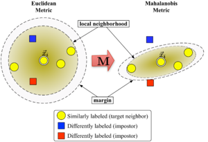
The algorithm distinguishes between two types of special data points: target neighbors and impostors.

Target neighbors

Target neighbors are selected before learning. Each instance ${\vec {x}}_{i}$ has exactly $k$ different target neighbors within $D$ , which all share the same class label $y_{i}$ . The target neighbors are the data points that should become nearest neighbors under the learned metric. Let us denote the set of target neighbors for a data point ${\vec {x}}_{i}$ as $N_{i}$ .

Impostors

An impostor of a data point ${\vec {x}}_{i}$ is another data point ${\vec {x}}_{j}$ with a different class label (i.e. $y_{i}\neq y_{j}$ ) which is one of the nearest neighbors of ${\vec {x}}_{i}$ . During learning the algorithm tries to minimize the number of impostors for all data instances in the training set.

Algorithm

Large margin nearest neighbors optimizes the matrix $\mathbf {M}$ with the help of semidefinite programming. The objective is twofold: For every data point ${\vec {x}}_{i}$ , the target neighbors should be close and the impostors should be far away. Figure 1 shows the effect of such an optimization on an illustrative example. The learned metric causes the input vector ${\vec {x}}_{i}$ to be surrounded by training instances of the same class. If it was a test point, it would be classified correctly under the $k=3$ nearest neighbor rule.

The first optimization goal is achieved by minimizing the average distance between instances and their target neighbors

\sum _{i,j\in N_{i}}d({\vec {x}}_{i},{\vec {x}}_{j})

The second goal is achieved by penalizing distances to impostors ${\vec {x}}_{l}$ that are less than one unit further away than target neighbors ${\vec {x}}_{j}$ (and therefore pushing them out of the local neighborhood of ${\vec {x}}_{i}$ ). The resulting value to be minimized can be stated as:

\sum _{i,j\in N_{i},l,y_{l}\neq y_{i}}[d({\vec {x}}_{i},{\vec {x}}_{j})+1-d({\vec {x}}_{i},{\vec {x}}_{l})]_{+}

With a hinge loss function ${\textstyle [\cdot ]_{+}=\max(\cdot ,0)}$ , which ensures that impostor proximity is not penalized when outside the margin. The margin of exactly one unit fixes the scale of the matrix $M$ . Any alternative choice $c>0$ would result in a rescaling of $M$ by a factor of $1/c$ .

The final optimization problem becomes:

\min _{\mathbf {M} }\sum _{i,j\in N_{i}}d({\vec {x}}_{i},{\vec {x}}_{j})+\lambda \sum _{i,j,l}\xi _{ijl}

\forall _{i,j\in N_{i},l,y_{l}\neq y_{i}}

d({\vec {x}}_{i},{\vec {x}}_{j})+1-d({\vec {x}}_{i},{\vec {x}}_{l})\leq \xi _{ijl}

\xi _{ijl}\geq 0

\mathbf {M} \succeq 0

The hyperparameter ${\textstyle \lambda >0}$ is some positive constant (typically set through cross-validation). Here the variables $\xi _{ijl}$ (together with two types of constraints) replace the term in the cost function. They play a role similar to slack variables to absorb the extent of violations of the impostor constraints. The last constraint ensures that $\mathbf {M}$ is positive semi-definite. The optimization problem is an instance of semidefinite programming (SDP). Although SDPs tend to suffer from high computational complexity, this particular SDP instance can be solved very efficiently due to the underlying geometric properties of the problem. In particular, most impostor constraints are naturally satisfied and do not need to be enforced during runtime (i.e. the set of variables $\xi _{ijl}$ is sparse). A particularly well suited solver technique is the working set method, which keeps a small set of constraints that are actively enforced and monitors the remaining (likely satisfied) constraints only occasionally to ensure correctness.

Extensions and efficient solvers

LMNN was extended to multiple local metrics in the 2008 paper.^[2] This extension significantly improves the classification error, but involves a more expensive optimization problem. In their 2009 publication in the Journal of Machine Learning Research,^[3] Weinberger and Saul derive an efficient solver for the semi-definite program. It can learn a metric for the MNIST handwritten digit data set in several hours, involving billions of pairwise constraints. An open source Matlab implementation is freely available at the authors web page.

Kumal et al.^[4] extended the algorithm to incorporate local invariances to multivariate polynomial transformations and improved regularization.

References

^ Weinberger, K. Q.; Blitzer J. C.; Saul L. K. (2006). "Distance Metric Learning for Large Margin Nearest Neighbor Classification". Advances in Neural Information Processing Systems. 18: 1473–1480.
^ Weinberger, K. Q.; Saul L. K. (2008). "Fast solvers and efficient implementations for distance metric learning" (PDF). Proceedings of International Conference on Machine Learning: 1160–1167. Archived from the original (PDF) on 2011-07-24. Retrieved 2010-07-14.
^ Weinberger, K. Q.; Saul L. K. (2009). "Distance Metric Learning for Large Margin Classification" (PDF). Journal of Machine Learning Research. 10: 207–244.
^ Kumar, M.P.; Torr P.H.S.; Zisserman A. (2007). "An Invariant Large Margin Nearest Neighbour Classifier". 2007 IEEE 11th International Conference on Computer Vision. pp. 1–8. doi:10.1109/ICCV.2007.4409041. ISBN 978-1-4244-1630-1. S2CID 1326101.

External links

This page was last edited on 24 July 2023, at 06:25

From Wikipedia, the free encyclopedia