Stable distribution

In probability theory, a distribution is said to be stable if a linear combination of two independent random variables with this distribution has the same distribution, up to location and scale parameters. A random variable is said to be stable if its distribution is stable. The stable distribution family is also sometimes referred to as the Lévy alpha-stable distribution, after Paul Lévy, the first mathematician to have studied it.^[1][2]

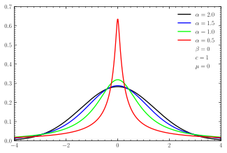
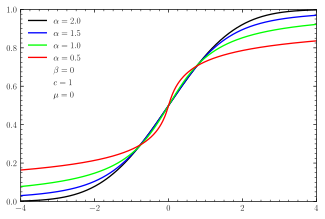
Of the four parameters defining the family, most attention has been focused on the stability parameter, ${\displaystyle \alpha }$ (see panel). Stable distributions have ${\displaystyle 0<\alpha \leq 2}$, with the upper bound corresponding to the normal distribution, and ${\displaystyle \alpha =1}$ to the Cauchy distribution. The distributions have undefined variance for ${\displaystyle \alpha <2}$, and undefined mean for ${\displaystyle \alpha \leq 1}$. The importance of stable probability distributions is that they are "attractors" for properly normed sums of independent and identically distributed (iid) random variables. The normal distribution defines a family of stable distributions. By the classical central limit theorem the properly normed sum of a set of random variables, each with finite variance, will tend toward a normal distribution as the number of variables increases. Without the finite variance assumption, the limit may be a stable distribution that is not normal. Mandelbrot referred to such distributions as "stable Paretian distributions",^[3][4][5] after Vilfredo Pareto. In particular, he referred to those maximally skewed in the positive direction with ${\displaystyle 1<\alpha <2}$ as "Pareto–Lévy distributions",^[1] which he regarded as better descriptions of stock and commodity prices than normal distributions.^[6]

Definition

A non-degenerate distribution is a stable distribution if it satisfies the following property:

Since the normal distribution, the Cauchy distribution, and the Lévy distribution all have the above property, it follows that they are special cases of stable distributions.

Such distributions form a four-parameter family of continuous probability distributions parametrized by location and scale parameters μ and c, respectively, and two shape parameters ${\displaystyle \beta }$ and ${\displaystyle \alpha }$, roughly corresponding to measures of asymmetry and concentration, respectively (see the figures).

The characteristic function ${\displaystyle \varphi (t)}$ of any probability distribution is the Fourier transform of its probability density function ${\displaystyle f(x)}$. The density function is therefore the inverse Fourier transform of the characteristic function:^[8]

Although the probability density function for a general stable distribution cannot be written analytically, the general characteristic function can be expressed analytically. A random variable X is called stable if its characteristic function can be written as^[7][9]

where sgn(t) is just the sign of t and μ ∈ R is a shift parameter, ${\displaystyle \beta \in [-1,1]}$, called the skewness parameter, is a measure of asymmetry. Notice that in this context the usual skewness is not well defined, as for ${\displaystyle \alpha <2}$ the distribution does not admit 2nd or higher moments, and the usual skewness definition is the 3rd central moment.

The reason this gives a stable distribution is that the characteristic function for the sum of two independent random variables equals the product of the two corresponding characteristic functions. Adding two random variables from a stable distribution gives something with the same values of ${\displaystyle \alpha }$ and ${\displaystyle \beta }$, but possibly different values of μ and c.

Not every function is the characteristic function of a legitimate probability distribution (that is, one whose cumulative distribution function is real and goes from 0 to 1 without decreasing), but the characteristic functions given above will be legitimate so long as the parameters are in their ranges. The value of the characteristic function at some value t is the complex conjugate of its value at −t as it should be so that the probability distribution function will be real.

In the simplest case ${\displaystyle \beta =0}$, the characteristic function is just a stretched exponential function; the distribution is symmetric about μ and is referred to as a (Lévy) symmetric alpha-stable distribution, often abbreviated SαS.

When ${\displaystyle \alpha <1}$ and ${\displaystyle \beta =1}$, the distribution is supported on [μ, ∞).

The parameter c > 0 is a scale factor which is a measure of the width of the distribution while ${\displaystyle \alpha }$ is the exponent or index of the distribution and specifies the asymptotic behavior of the distribution.

Parametrizations

The above definition is only one of the parametrizations in use for stable distributions; it is the most common but its probability density is not continuous in the parameters at ${\displaystyle \alpha =1}$.^[10]

A continuous parametrization is^[7]

where:

The ranges of ${\displaystyle \alpha }$ and ${\displaystyle \beta }$ are the same as before, γ (like c) should be positive, and δ (like μ) should be real.

In either parametrization one can make a linear transformation of the random variable to get a random variable whose density is ${\displaystyle f(y;\alpha ,\beta ,1,0)}$. In the first parametrization, this is done by defining the new variable:

For the second parametrization, simply use

no matter what ${\displaystyle \alpha }$ is. In the first parametrization, if the mean exists (that is, ${\displaystyle \alpha >1}$) then it is equal to μ, whereas in the second parametrization when the mean exists it is equal to ${\displaystyle \delta -\beta \gamma \tan \left({\tfrac {\pi \alpha }{2}}\right).}$

The distribution

A stable distribution is therefore specified by the above four parameters. It can be shown that any non-degenerate stable distribution has a smooth (infinitely differentiable) density function.^[7] If ${\displaystyle f(x;\alpha ,\beta ,c,\mu )}$ denotes the density of X and Y is the sum of independent copies of X:

then Y has the density ${\displaystyle {\tfrac {1}{s}}f(y/s;\alpha ,\beta ,c,0)}$ with

The asymptotic behavior is described, for ${\displaystyle \alpha <2}$, by:^[7]

where Γ is the Gamma function (except that when ${\displaystyle \alpha \geq 1}$ and ${\displaystyle \beta =\pm 1}$, the tail does not vanish to the left or right, resp., of μ, although the above expression is 0). This "heavy tail" behavior causes the variance of stable distributions to be infinite for all ${\displaystyle \alpha <2}$. This property is illustrated in the log–log plots below.

When ${\displaystyle \alpha =2}$, the distribution is Gaussian (see below), with tails asymptotic to exp(−x²/4c²)/(2c√π).

One-sided stable distribution and stable count distribution

When ${\displaystyle \alpha <1}$ and ${\displaystyle \beta =1}$, the distribution is supported on [μ, ∞). This family is called one-sided stable distribution.^[11] Its standard distribution (μ=0) is defined as

${\displaystyle L_{\alpha }(x)=f{\left(x;\alpha ,1,\cos \left({\frac {\alpha \pi }{2}}\right)^{1/\alpha },0\right)}}$, where ${\displaystyle \alpha <1}$.

Let ${\displaystyle q=\exp(-i\alpha \pi /2)}$, its characteristic function is ${\displaystyle \varphi (t;\alpha )=\exp \left(-q|t|^{\alpha }\right)}$. Thus the integral form of its PDF is (note: ${\displaystyle \operatorname {Im} (q)<0}$)

The double-sine integral is more effective for very small ${\displaystyle x}$.

Consider the Lévy sum ${\textstyle Y=\sum _{i=1}^{N}X_{i}}$ where ${\textstyle X_{i}\sim L_{\alpha }(x)}$, then Y has the density ${\textstyle {\frac {1}{\nu }}L_{\alpha }{\left({\frac {x}{\nu }}\right)}}$ where ${\textstyle \nu =N^{1/\alpha }}$. Set ${\textstyle x=1}$ to arrive at the stable count distribution.^[12] Its standard distribution is defined as

${\displaystyle {\mathfrak {N}}_{\alpha }(\nu )={\frac {\alpha }{\Gamma \left({\frac {1}{\alpha }}\right)}}{\frac {1}{\nu }}L_{\alpha }{\left({\frac {1}{\nu }}\right)}}$, where ${\displaystyle \nu >0}$ and ${\displaystyle \alpha <1}$.

The stable count distribution is the conjugate prior of the one-sided stable distribution. Its location-scale family is defined as

${\displaystyle {\mathfrak {N}}_{\alpha }(\nu ;\nu _{0},\theta )={\frac {\alpha }{\Gamma ({\frac {1}{\alpha }})}}{\frac {1}{\nu -\nu _{0}}}L_{\alpha }{\left({\frac {\theta }{\nu -\nu _{0}}}\right)}}$, where ${\displaystyle \nu >\nu _{0}}$, ${\displaystyle \theta >0}$, and ${\displaystyle \alpha <1}$.

It is also a one-sided distribution supported on ${\displaystyle [\nu _{0},\infty )}$. The location parameter ${\displaystyle \nu _{0}}$ is the cut-off location, while ${\displaystyle \theta }$ defines its scale.

When ${\textstyle \alpha ={\frac {1}{2}}}$, ${\textstyle L_{\frac {1}{2}}(x)}$ is the Lévy distribution which is an inverse gamma distribution. Thus ${\displaystyle {\mathfrak {N}}_{\frac {1}{2}}(\nu ;\nu _{0},\theta )}$ is a shifted gamma distribution of shape 3/2 and scale ${\displaystyle 4\theta }$,

${\displaystyle {\mathfrak {N}}_{\frac {1}{2}}(\nu ;\nu _{0},\theta )={\frac {1}{4{\sqrt {\pi }}\theta ^{3/2}}}(\nu -\nu _{0})^{1/2}e^{-{\frac {\nu -\nu _{0}}{4\theta }}}}$, where ${\displaystyle \nu >\nu _{0}}$, ${\displaystyle \theta >0}$.

Its mean is ${\displaystyle \nu _{0}+6\theta }$ and its standard deviation is ${\displaystyle {\sqrt {24}}\theta }$. It is hypothesized that VIX is distributed like ${\textstyle {\mathfrak {N}}_{\frac {1}{2}}(\nu ;\nu _{0},\theta )}$ with ${\displaystyle \nu _{0}=10.4}$ and ${\displaystyle \theta =1.6}$ (See Section 7 of ^[12]). Thus the stable count distribution is the first-order marginal distribution of a volatility process. In this context, ${\displaystyle \nu _{0}}$ is called the "floor volatility".

Another approach to derive the stable count distribution is to use the Laplace transform of the one-sided stable distribution, (Section 2.4 of ^[12])

${\displaystyle \int _{0}^{\infty }e^{-zx}L_{\alpha }(x)dx=e^{-z^{\alpha }}}$, where ${\displaystyle \alpha <1}$.

Let ${\displaystyle x=1/\nu }$, and one can decompose the integral on the left hand side as a product distribution of a standard Laplace distribution and a standard stable count distribution,f

${\displaystyle \int _{0}^{\infty }{\frac {1}{\nu }}\left({\frac {1}{2}}e^{-{\frac {|z|}{\nu }}}\right)\left({\frac {\alpha }{\Gamma ({\frac {1}{\alpha }})}}{\frac {1}{\nu }}L_{\alpha }{\left({\frac {1}{\nu }}\right)}\right)d\nu ={\frac {1}{2}}{\frac {\alpha }{\Gamma ({\frac {1}{\alpha }})}}e^{-|z|^{\alpha }}}$, where ${\displaystyle \alpha <1}$.

This is called the "lambda decomposition" (See Section 4 of ^[12]) since the right hand side was named as "symmetric lambda distribution" in Lihn's former works. However, it has several more popular names such as "exponential power distribution", or the "generalized error/normal distribution", often referred to when ${\displaystyle \alpha >1}$.

The n-th moment of ${\displaystyle {\mathfrak {N}}_{\alpha }(\nu )}$ is the ${\displaystyle -(n+1)}$-th moment of ${\displaystyle L_{\alpha }(x)}$, and all positive moments are finite.

Properties

• All stable distributions are infinitely divisible.
• With the exception of the normal distribution (${\displaystyle \alpha =2}$), stable distributions are leptokurtotic and heavy-tailed distributions.
• Closure under convolution

Stable distributions are closed under convolution for a fixed value of ${\displaystyle \alpha }$. Since convolution is equivalent to multiplication of the Fourier-transformed function, it follows that the product of two stable characteristic functions with the same ${\displaystyle \alpha }$ will yield another such characteristic function. The product of two stable characteristic functions is given by:

Since Φ is not a function of the μ, c or ${\displaystyle \beta }$ variables it follows that these parameters for the convolved function are given by:

In each case, it can be shown that the resulting parameters lie within the required intervals for a stable distribution.

The Generalized Central Limit Theorem

The Generalized Central Limit Theorem (GCLT) was an effort of multiple mathematicians (Berstein, Lindeberg, Lévy, Feller, Kolmogorov, and others) over the period from 1920 to 1937. ^[13] The first published complete proof (in French) of the GCLT was in 1937 by Paul Lévy.^[14] An English language version of the complete proof of the GCLT is available in the translation of Gnedenko and Kolmogorov's 1954 book.^[15]

The statement of the GLCT is as follows:^[16]

A non-degenerate random variable Z is α-stable for some 0 < α ≤ 2 if and only if there is an independent, identically distributed sequence of random variables X₁, X₂, X₃, ... and constants a_n > 0, b_n ∈ ℝ with

a_n (X₁ + ... + X_n) - b_n → Z.

Here → means the sequence of random variable sums converges in distribution; i.e., the corresponding distributions satisfy F_n(y) → F(y) at all continuity points of F.

In other words, if sums of independent, identically distributed random variables converge in distribution to some Z, then Z must be a stable distribution.

A generalized central limit theorem

General reference: ^[17] by Gnedenko.

Another important property of stable distributions is the role that they play in a generalized central limit theorem. The central limit theorem states that the sum of a number of independent and identically distributed (i.i.d.) random variables with finite non-zero variances will tend to a normal distribution as the number of variables grows.

A generalization due to Gnedenko and Kolmogorov states that the sum of a number of random variables with symmetric distributions having power-law tails (Paretian tails), decreasing as ${\displaystyle |x|^{-\alpha -1}}$ where ${\displaystyle 0<\alpha \leqslant 2}$ (and therefore having infinite variance), will tend to a stable distribution ${\displaystyle f(x;\alpha ,0,c,0)}$ as the number of summands grows.^[18] If ${\displaystyle \alpha >2}$ then the sum converges to a stable distribution with stability parameter equal to 2, i.e. a Gaussian distribution.^[19]

^[20]

There are other possibilities as well. For example, if the characteristic function of the random variable is asymptotic to ${\displaystyle 1+a|t|^{\alpha }\ln |t|}$ for small t (positive or negative), then we may ask how t varies with n when the value of the characteristic function for the sum of n such random variables equals a given value u:

Assuming for the moment that t → 0, take the limit of the above as n → ∞:

Therefore:

This shows that ${\displaystyle \ln |t|}$ is asymptotic to ${\displaystyle {\tfrac {-1}{\alpha }}\ln n,}$ so using the previous equation this leads to

This implies that the sum divided by

has a characteristic function whose value at some t′ goes to u (as n increases) when ${\displaystyle t'=(-\ln u)^{{1}/{\alpha }}.}$ In other words, the characteristic function converges pointwise to ${\displaystyle \exp(-(t')^{\alpha })}$ and therefore by Lévy's continuity theorem the sum divided by

converges in distribution to the symmetric alpha-stable distribution with stability parameter ${\displaystyle \alpha }$ and scale parameter 1.

This can be applied to a random variable whose tails decrease as ${\displaystyle |x|^{-3}}$. This random variable has a mean but the variance is infinite. Let us take the following distribution:

This can be written as

where

We want to find the leading terms of the asymptotic expansion of the characteristic function. The characteristic function of the probability distribution ${\textstyle {\frac {1}{w}}h\left({\frac {x}{w}}\right)}$ is ${\textstyle {\tfrac {\sin(tw)}{tw}},}$ so the characteristic function for f(x) is

and calculate: where ${\displaystyle C_{1},C_{2}}$ and ${\displaystyle C_{3}}$ are constants. Therefore, and according to what was said above (and the fact that the variance of f(x;2,0,1,0) is 2), the sum of n instances of this random variable, divided by ${\textstyle {\sqrt {n(\ln n)/12}},}$ will converge in distribution to a Gaussian distribution with variance 1. But the variance at any particular n will still be infinite. Note that the width of the limiting distribution grows faster than in the case where the random variable has a finite variance (in which case the width grows as the square root of n). The average, obtained by dividing the sum by n, tends toward a Gaussian whose width approaches zero as n increases, in accordance with the Law of large numbers.

Special cases

There is no general analytic solution for the form of f(x). There are, however three special cases which can be expressed in terms of elementary functions as can be seen by inspection of the characteristic function:^[7][9][21]

• For ${\displaystyle \alpha =2}$ the distribution reduces to a Gaussian distribution with variance σ² = 2c² and mean μ; the skewness parameter ${\displaystyle \beta }$ has no effect.
• For ${\displaystyle \alpha =1}$ and ${\displaystyle \beta =0}$ the distribution reduces to a Cauchy distribution with scale parameter c and shift parameter μ.
• For ${\displaystyle \alpha =1/2}$ and ${\displaystyle \beta =1}$ the distribution reduces to a Lévy distribution with scale parameter c and shift parameter μ.

Note that the above three distributions are also connected, in the following way: A standard Cauchy random variable can be viewed as a mixture of Gaussian random variables (all with mean zero), with the variance being drawn from a standard Lévy distribution. And in fact this is a special case of a more general theorem (See p. 59 of ^[22]) which allows any symmetric alpha-stable distribution to be viewed in this way (with the alpha parameter of the mixture distribution equal to twice the alpha parameter of the mixing distribution—and the beta parameter of the mixing distribution always equal to one).

A general closed form expression for stable PDFs with rational values of ${\displaystyle \alpha }$ is available in terms of Meijer G-functions.^[23] Fox H-Functions can also be used to express the stable probability density functions. For simple rational numbers, the closed form expression is often in terms of less complicated special functions. Several closed form expressions having rather simple expressions in terms of special functions are available. In the table below, PDFs expressible by elementary functions are indicated by an E and those that are expressible by special functions are indicated by an s.^[22]

		${\displaystyle \alpha }$
		1/3	1/2	2/3	1	4/3	3/2	2
${\displaystyle \beta }$	0	s	s	s	E	s	s	E
	1	s	E	s	L		s

Some of the special cases are known by particular names:

• For ${\displaystyle \alpha =1}$ and ${\displaystyle \beta =1}$, the distribution is a Landau distribution (L) which has a specific usage in physics under this name.
• For ${\displaystyle \alpha =3/2}$ and ${\displaystyle \beta =0}$ the distribution reduces to a Holtsmark distribution with scale parameter c and shift parameter μ.

Also, in the limit as c approaches zero or as α approaches zero the distribution will approach a Dirac delta function δ(x − μ).

Series representation

The stable distribution can be restated as the real part of a simpler integral:^[24]

Expressing the second exponential as a Taylor series, this leads to:

where ${\displaystyle q=c^{\alpha }(1-i\beta \Phi )}$. Reversing the order of integration and summation, and carrying out the integration yields: which will be valid for x ≠ μ and will converge for appropriate values of the parameters. (Note that the n = 0 term which yields a delta function in x − μ has therefore been dropped.) Expressing the first exponential as a series will yield another series in positive powers of x − μ which is generally less useful.

For one-sided stable distribution, the above series expansion needs to be modified, since ${\displaystyle q=\exp(-i\alpha \pi /2)}$ and ${\displaystyle qi^{\alpha }=1}$. There is no real part to sum. Instead, the integral of the characteristic function should be carried out on the negative axis, which yields:^[25][11]

Simulation of stable variables

Simulating sequences of stable random variables is not straightforward, since there are no analytic expressions for the inverse ${\displaystyle F^{-1}(x)}$ nor the CDF ${\displaystyle F(x)}$ itself.^[10][12] All standard approaches like the rejection or the inversion methods would require tedious computations. A much more elegant and efficient solution was proposed by Chambers, Mallows and Stuck (CMS),^[26] who noticed that a certain integral formula^[27] yielded the following algorithm:^[28]

• generate a random variable ${\displaystyle U}$ uniformly distributed on ${\displaystyle \left(-{\tfrac {\pi }{2}},{\tfrac {\pi }{2}}\right)}$ and an independent exponential random variable ${\displaystyle W}$ with mean 1;
• for ${\displaystyle \alpha \neq 1}$ compute:
  $${\displaystyle X=\left(1+\zeta ^{2}\right)^{\frac {1}{2\alpha }}{\frac {\sin(\alpha (U+\xi ))}{(\cos(U))^{\frac {1}{\alpha }}}}\left({\frac {\cos(U-\alpha (U+\xi ))}{W}}\right)^{\frac {1-\alpha }{\alpha }},}$$

  
• for ${\displaystyle \alpha =1}$ compute:
  $${\displaystyle X={\frac {1}{\xi }}\left\{\left({\frac {\pi }{2}}+\beta U\right)\tan U-\beta \log \left({\frac {{\frac {\pi }{2}}W\cos U}{{\frac {\pi }{2}}+\beta U}}\right)\right\},}$$

  
  where
  $${\displaystyle \zeta =-\beta \tan {\frac {\pi \alpha }{2}},\qquad \xi ={\begin{cases}{\frac {1}{\alpha }}\arctan(-\zeta )&\alpha \neq 1\\{\frac {\pi }{2}}&\alpha =1\end{cases}}}$$

  

This algorithm yields a random variable ${\displaystyle X\sim S_{\alpha }(\beta ,1,0)}$. For a detailed proof see.^[29]

Given the formulas for simulation of a standard stable random variable, we can easily simulate a stable random variable for all admissible values of the parameters ${\displaystyle \alpha }$, ${\displaystyle c}$, ${\displaystyle \beta }$ and ${\displaystyle \mu }$ using the following property. If ${\displaystyle X\sim S_{\alpha }(\beta ,1,0)}$ then

is ${\displaystyle S_{\alpha }(\beta ,c,\mu )}$. For ${\displaystyle \alpha =2}$ (and ${\displaystyle \beta =0}$) the CMS method reduces to the well known Box-Muller transform for generating Gaussian random variables.^[30] Many other approaches have been proposed in the literature, including application of Bergström^[31] and LePage^[32] series expansions. However, the CMS method is regarded as the fastest and the most accurate.

Applications

Stable distributions owe their importance in both theory and practice to the generalization of the central limit theorem to random variables without second (and possibly first) order moments and the accompanying self-similarity of the stable family. It was the seeming departure from normality along with the demand for a self-similar model for financial data (i.e. the shape of the distribution for yearly asset price changes should resemble that of the constituent daily or monthly price changes) that led Benoît Mandelbrot to propose that cotton prices follow an alpha-stable distribution with ${\displaystyle \alpha }$ equal to 1.7.^[6] Lévy distributions are frequently found in analysis of critical behavior and financial data.^[9][33]

They are also found in spectroscopy as a general expression for a quasistatically pressure broadened spectral line.^[24]

The Lévy distribution of solar flare waiting time events (time between flare events) was demonstrated for CGRO BATSE hard x-ray solar flares in December 2001. Analysis of the Lévy statistical signature revealed that two different memory signatures were evident; one related to the solar cycle and the second whose origin appears to be associated with a localized or combination of localized solar active region effects.^[34]

Other analytic cases

A number of cases of analytically expressible stable distributions are known. Let the stable distribution be expressed by ${\displaystyle f(x;\alpha ,\beta ,c,\mu )}$, then:

• The Cauchy Distribution is given by ${\displaystyle f(x;1,0,1,0).}$
• The Lévy distribution is given by ${\displaystyle f(x;{\tfrac {1}{2}},1,1,0).}$
• The Normal distribution is given by ${\displaystyle f(x;2,0,1,0).}$
• Let ${\displaystyle S_{\mu ,\nu }(z)}$ be a Lommel function, then:^[35]
  $${\displaystyle f\left(x;{\tfrac {1}{3}},0,1,0\right)=\Re \left({\frac {2e^{-{\frac {i\pi }{4}}}}{3{\sqrt {3}}\pi }}{\frac {1}{\sqrt {x^{3}}}}S_{0,{\frac {1}{3}}}\left({\frac {2e^{\frac {i\pi }{4}}}{3{\sqrt {3}}}}{\frac {1}{\sqrt {x}}}\right)\right)}$$

  
• Let ${\displaystyle S(x)}$ and ${\displaystyle C(x)}$ denote the Fresnel integrals, then:^[36]
  $${\displaystyle f\left(x;{\tfrac {1}{2}},0,1,0\right)={\frac {1}{\sqrt {2\pi |x|^{3}}}}\left(\sin \left({\tfrac {1}{4|x|}}\right)\left[{\frac {1}{2}}-S\left({\tfrac {1}{\sqrt {2\pi |x|}}}\right)\right]+\cos \left({\tfrac {1}{4|x|}}\right)\left[{\frac {1}{2}}-C\left({\tfrac {1}{\sqrt {2\pi |x|}}}\right)\right]\right)}$$

  
• Let ${\displaystyle K_{v}(x)}$ be the modified Bessel function of the second kind, then:^[36]
  $${\displaystyle f\left(x;{\tfrac {1}{3}},1,1,0\right)={\frac {1}{\pi }}{\frac {2{\sqrt {2}}}{3^{\frac {7}{4}}}}{\frac {1}{\sqrt {x^{3}}}}K_{\frac {1}{3}}\left({\frac {4{\sqrt {2}}}{3^{\frac {9}{4}}}}{\frac {1}{\sqrt {x}}}\right)}$$

  
• If the ${\displaystyle {}_{m}F_{n}}$ denote the hypergeometric functions, then:^[35]
  $${\displaystyle {\begin{aligned}f\left(x;{\tfrac {4}{3}},0,1,0\right)&={\frac {3^{\frac {5}{4}}}{4{\sqrt {2\pi }}}}{\frac {\Gamma \left({\tfrac {7}{12}}\right)\Gamma \left({\tfrac {11}{12}}\right)}{\Gamma \left({\tfrac {6}{12}}\right)\Gamma \left({\tfrac {8}{12}}\right)}}{}_{2}F_{2}\left({\tfrac {7}{12}},{\tfrac {11}{12}};{\tfrac {6}{12}},{\tfrac {8}{12}};{\tfrac {3^{3}x^{4}}{4^{4}}}\right)-{\frac {3^{\frac {11}{4}}x^{3}}{4^{3}{\sqrt {2\pi }}}}{\frac {\Gamma \left({\tfrac {13}{12}}\right)\Gamma \left({\tfrac {17}{12}}\right)}{\Gamma \left({\tfrac {18}{12}}\right)\Gamma \left({\tfrac {15}{12}}\right)}}{}_{2}F_{2}\left({\tfrac {13}{12}},{\tfrac {17}{12}};{\tfrac {18}{12}},{\tfrac {15}{12}};{\tfrac {3^{3}x^{4}}{4^{4}}}\right)\\[6pt]f\left(x;{\tfrac {3}{2}},0,1,0\right)&={\frac {\Gamma \left({\tfrac {5}{3}}\right)}{\pi }}{}_{2}F_{3}\left({\tfrac {5}{12}},{\tfrac {11}{12}};{\tfrac {1}{3}},{\tfrac {1}{2}},{\tfrac {5}{6}};-{\tfrac {2^{2}x^{6}}{3^{6}}}\right)-{\frac {x^{2}}{3\pi }}{}_{3}F_{4}\left({\tfrac {3}{4}},1,{\tfrac {5}{4}};{\tfrac {2}{3}},{\tfrac {5}{6}},{\tfrac {7}{6}},{\tfrac {4}{3}};-{\tfrac {2^{2}x^{6}}{3^{6}}}\right)+{\frac {7x^{4}\Gamma \left({\tfrac {4}{3}}\right)}{3^{4}\pi ^{2}}}{}_{2}F_{3}\left({\tfrac {13}{12}},{\tfrac {19}{12}};{\tfrac {7}{6}},{\tfrac {3}{2}},{\tfrac {5}{3}};-{\tfrac {2^{2}x^{6}}{3^{6}}}\right)\end{aligned}}}$$

  
  with the latter being the Holtsmark distribution.
• Let ${\displaystyle W_{k,\mu }(z)}$ be a Whittaker function, then:^[37][38][39]
  $${\displaystyle {\begin{aligned}f\left(x;{\tfrac {2}{3}},0,1,0\right)&={\frac {\sqrt {3}}{6{\sqrt {\pi }}|x|}}\exp \left({\tfrac {2}{27}}x^{-2}\right)W_{-{\frac {1}{2}},{\frac {1}{6}}}\left({\tfrac {4}{27}}x^{-2}\right)\\[8pt]f\left(x;{\tfrac {2}{3}},1,1,0\right)&={\frac {\sqrt {3}}{{\sqrt {\pi }}|x|}}\exp \left(-{\tfrac {16}{27}}x^{-2}\right)W_{{\frac {1}{2}},{\frac {1}{6}}}\left({\tfrac {32}{27}}x^{-2}\right)\\[8pt]f\left(x;{\tfrac {3}{2}},1,1,0\right)&={\begin{cases}{\frac {\sqrt {3}}{{\sqrt {\pi }}|x|}}\exp \left({\frac {1}{27}}x^{3}\right)W_{{\frac {1}{2}},{\frac {1}{6}}}\left(-{\frac {2}{27}}x^{3}\right)&x<0\\{}\\{\frac {\sqrt {3}}{6{\sqrt {\pi }}|x|}}\exp \left({\frac {1}{27}}x^{3}\right)W_{-{\frac {1}{2}},{\frac {1}{6}}}\left({\frac {2}{27}}x^{3}\right)&x\geq 0\end{cases}}\end{aligned}}}$$

  

See also

• Lévy flight
• Lévy process
• Other "power law" distributions
  • Pareto distribution
  • Zeta distribution
  • Zipf distribution
  • Zipf–Mandelbrot distribution
• Financial models with long-tailed distributions and volatility clustering
• Multivariate stable distribution
• Discrete-stable distribution

Notes

• The STABLE program for Windows is available from John Nolan's stable webpage: http://www.robustanalysis.com/public/stable.html. It calculates the density (pdf), cumulative distribution function (cdf) and quantiles for a general stable distribution, and performs maximum likelihood estimation of stable parameters and some exploratory data analysis techniques for assessing the fit of a data set.
• libstable is a C implementation for the Stable distribution pdf, cdf, random number, quantile and fitting functions (along with a benchmark replication package and an R package).
• R Package 'stabledist'  by Diethelm Wuertz, Martin Maechler and Rmetrics core team members. Computes stable density, probability, quantiles, and random numbers. Updated Sept. 12, 2016.
• Python implementation is located in scipy.stats.levy_stable in the SciPy package.
• Julia provides package StableDistributions.jl which has methods of generation, fitting, probability density, cumulative distribution function, characteristic and moment generating functions, quantile and related functions, convolution and affine transformations of stable distributions. It uses modernised algorithms improved by John P. Nolan.^[16]

References

^ abMandelbrot, B. (1960). "The Pareto–Lévy Law and the Distribution of Income". International Economic Review. 1 (2): 79–106. doi:10.2307/2525289. JSTOR2525289.
^Lévy, Paul (1925). Calcul des probabilités. Paris: Gauthier-Villars. OCLC1417531.
^Mandelbrot, B. (1961). "Stable Paretian Random Functions and the Multiplicative Variation of Income". Econometrica. 29 (4): 517–543. doi:10.2307/1911802. JSTOR1911802.
^Mandelbrot, B. (1963). "The Variation of Certain Speculative Prices". The Journal of Business. 36 (4): 394–419. doi:10.1086/294632. JSTOR2350970.
^Fama, Eugene F. (1963). "Mandelbrot and the Stable Paretian Hypothesis". The Journal of Business. 36 (4): 420–429. doi:10.1086/294633. JSTOR2350971.
^ abcVoit, Johannes (2005). Balian, R; Beiglböck, W; Grosse, H; Thirring, W (eds.). The Statistical Mechanics of Financial Markets – Springer. Texts and Monographs in Physics. Springer. doi:10.1007/b137351. ISBN978-3-540-26285-5.
^ abNolan, John P. (1997). "Numerical calculation of stable densities and distribution functions". Communications in Statistics. Stochastic Models. 13 (4): 759–774. doi:10.1080/15326349708807450. ISSN0882-0287.
^Lévy, Paul (1937). Theorie de l'addition des variables aleatoires [Combination theory of unpredictable variables]. Paris: Gauthier-Villars.
^Gnedenko, Boris Vladimirovich; Kologorov, Andreĭ Nikolaevich; Doob, Joseph L.; Hsu, Pao-Lu (1968). Limit distributions for sums of independent random variables. Reading, MA: Addison-wesley.
^Gnedenko, Boris V. (2020-06-30). "10: The Theory of Infinitely Divisible Distributions". Theory of Probability (6th ed.). CRC Press. ISBN978-0-367-57931-9.
^Araujo, Aloisio; Giné, Evarist (1980). "Chapter 2". The central limit theorem for real and Banach valued random variables. Wiley series in probability and mathematical statistics. New York: Wiley. ISBN978-0-471-05304-0.
^Zolotarev, V. (1995). "On Representation of Densities of Stable Laws by Special Functions". Theory of Probability and Its Applications. 39 (2): 354–362. doi:10.1137/1139025. ISSN0040-585X.
^Chambers, J. M.; Mallows, C. L.; Stuck, B. W. (1976). "A Method for Simulating Stable Random Variables". Journal of the American Statistical Association. 71 (354): 340–344. doi:10.1080/01621459.1976.10480344. ISSN0162-1459.
^Janicki, Aleksander; Kokoszka, Piotr (1992). "Computer investigation of the Rate of Convergence of Lepage Type Series to α-Stable Random Variables". Statistics. 23 (4): 365–373. doi:10.1080/02331889208802383. ISSN0233-1888.
^ abGaroni, T. M.; Frankel, N. E. (2002). "Lévy flights: Exact results and asymptotics beyond all orders". Journal of Mathematical Physics. 43 (5): 2670–2689. Bibcode:2002JMP....43.2670G. doi:10.1063/1.1467095.
^Uchaikin, V. V.; Zolotarev, V. M. (1999). "Chance And Stability – Stable Distributions And Their Applications". VSP.
^Zlotarev, V. M. (1961). "Expression of the density of a stable distribution with exponent alpha greater than one by means of a frequency with exponent 1/alpha". Selected Translations in Mathematical Statistics and Probability (Translated from the Russian Article: Dokl. Akad. Nauk SSSR. 98, 735–738 (1954)). 1: 163–167.
![{\displaystyle \alpha \in (0,2]}](https://wikimedia.org/api/rest_v1/media/math/render/svg/98dade01a06507996c8330ec68b7c0f7bc305a05)
![{\displaystyle \exp \!{\Big [}\;it\mu -|c\,t|^{\alpha }\,(1-i\beta \operatorname {sgn}(t)\Phi )\;{\Big ]},}](https://wikimedia.org/api/rest_v1/media/math/render/svg/7d98d0e47ac7b119c61fcddb23c16046f082f0b5)
![{\displaystyle \beta \in [-1,1]}](https://wikimedia.org/api/rest_v1/media/math/render/svg/88346c1460c3477cc60acc78f4c9742e51770644)
![{\displaystyle {\begin{aligned}L_{\alpha }(x)&={\frac {1}{\pi }}\Re \left[\int _{-\infty }^{\infty }e^{itx}e^{-q|t|^{\alpha }}\,dt\right]\\&={\frac {2}{\pi }}\int _{0}^{\infty }e^{-\operatorname {Re} (q)\,t^{\alpha }}\sin(tx)\sin(-\operatorname {Im} (q)\,t^{\alpha })\,dt,{\text{ or }}\\&={\frac {2}{\pi }}\int _{0}^{\infty }e^{-{\text{Re}}(q)\,t^{\alpha }}\cos(tx)\cos(\operatorname {Im} (q)\,t^{\alpha })\,dt.\end{aligned}}}](https://wikimedia.org/api/rest_v1/media/math/render/svg/f81444eb51f2cc30ebea9ee2384018907c5d4d39)
![{\displaystyle {\begin{aligned}\mu &=\mu _{1}+\mu _{2}\\|c|&=\left(|c_{1}|^{\alpha }+|c_{2}|^{\alpha }\right)^{\frac {1}{\alpha }}\\[6pt]\beta &={\frac {\beta _{1}|c_{1}|^{\alpha }+\beta _{2}|c_{2}|^{\alpha }}{|c_{1}|^{\alpha }+|c_{2}|^{\alpha }}}\end{aligned}}}](https://wikimedia.org/api/rest_v1/media/math/render/svg/160e86b38cd71e522fc4ec9b6d51795e465dd9f0)
![{\displaystyle {\begin{aligned}\ln(\ln u)&=\ln \left(\lim _{n\to \infty }na|t|^{\alpha }\ln |t|\right)\\[5pt]&=\lim _{n\to \infty }\ln \left(na|t|^{\alpha }\ln |t|\right)=\lim _{n\to \infty }\left[\ln(na)+\alpha \ln |t|+\ln(\ln |t|)\right]\end{aligned}}}](https://wikimedia.org/api/rest_v1/media/math/render/svg/1f76b3b4f4b7f0bd7cbe616bfe81b50584665654)
![{\displaystyle {\begin{aligned}\varphi (t)-1&=\int _{1}^{\infty }{\frac {2}{w^{3}}}\left[{\frac {\sin(tw)}{tw}}-1\right]\,dw\\&=\int _{1}^{\frac {1}{|t|}}{\frac {2}{w^{3}}}\left[{\frac {\sin(tw)}{tw}}-1\right]\,dw+\int _{\frac {1}{|t|}}^{\infty }{\frac {2}{w^{3}}}\left[{\frac {\sin(tw)}{tw}}-1\right]\,dw\\&=\int _{1}^{\frac {1}{|t|}}{\frac {2}{w^{3}}}\left[{\frac {\sin(tw)}{tw}}-1+\left\{-{\frac {t^{2}w^{2}}{3!}}+{\frac {t^{2}w^{2}}{3!}}\right\}\right]\,dw+\int _{\frac {1}{|t|}}^{\infty }{\frac {2}{w^{3}}}\left[{\frac {\sin(tw)}{tw}}-1\right]\,dw\\&=\int _{1}^{\frac {1}{|t|}}-{\frac {t^{2}dw}{3w}}+\int _{1}^{\frac {1}{|t|}}{\frac {2}{w^{3}}}\left[{\frac {\sin(tw)}{tw}}-1+{\frac {t^{2}w^{2}}{3!}}\right]dw+\int _{\frac {1}{|t|}}^{\infty }{\frac {2}{w^{3}}}\left[{\frac {\sin(tw)}{tw}}-1\right]dw\\&=\int _{1}^{\frac {1}{|t|}}-{\frac {t^{2}dw}{3w}}+\left\{\int _{0}^{\frac {1}{|t|}}{\frac {2}{w^{3}}}\left[{\frac {\sin(tw)}{tw}}-1+{\frac {t^{2}w^{2}}{3!}}\right]dw-\int _{0}^{1}{\frac {2}{w^{3}}}\left[{\frac {\sin(tw)}{tw}}-1+{\frac {t^{2}w^{2}}{3!}}\right]dw\right\}+\int _{\frac {1}{|t|}}^{\infty }{\frac {2}{w^{3}}}\left[{\frac {\sin(tw)}{tw}}-1\right]dw\\&=\int _{1}^{\frac {1}{|t|}}-{\frac {t^{2}dw}{3w}}+t^{2}\int _{0}^{1}{\frac {2}{y^{3}}}\left[{\frac {\sin(y)}{y}}-1+{\frac {y^{2}}{6}}\right]dy-\int _{0}^{1}{\frac {2}{w^{3}}}\left[{\frac {\sin(tw)}{tw}}-1+{\frac {t^{2}w^{2}}{6}}\right]dw+t^{2}\int _{1}^{\infty }{\frac {2}{y^{3}}}\left[{\frac {\sin(y)}{y}}-1\right]dy\\&=-{\frac {t^{2}}{3}}\int _{1}^{\frac {1}{|t|}}{\frac {dw}{w}}+t^{2}C_{1}-\int _{0}^{1}{\frac {2}{w^{3}}}\left[{\frac {\sin(tw)}{tw}}-1+{\frac {t^{2}w^{2}}{6}}\right]dw+t^{2}C_{2}\\&={\frac {t^{2}}{3}}\ln |t|+t^{2}C_{3}-\int _{0}^{1}{\frac {2}{w^{3}}}\left[{\frac {\sin(tw)}{tw}}-1+{\frac {t^{2}w^{2}}{6}}\right]dw\\&={\frac {t^{2}}{3}}\ln |t|+t^{2}C_{3}-\int _{0}^{1}{\frac {2}{w^{3}}}\left[{\frac {t^{4}w^{4}}{5!}}+\cdots \right]dw\\&={\frac {t^{2}}{3}}\ln |t|+t^{2}C_{3}-{\mathcal {O}}\left(t^{4}\right)\end{aligned}}}](https://wikimedia.org/api/rest_v1/media/math/render/svg/1a37af99ace7b16378436ef24dc33e4162846bbf)
![{\displaystyle f(x;\alpha ,\beta ,c,\mu )={\frac {1}{\pi }}\Re \left[\int _{0}^{\infty }e^{it(x-\mu )}e^{-(ct)^{\alpha }(1-i\beta \Phi )}\,dt\right].}](https://wikimedia.org/api/rest_v1/media/math/render/svg/0d6b466b832c1e998c2bfa0c4960b0219910a438)
![{\displaystyle f(x;\alpha ,\beta ,c,\mu )={\frac {1}{\pi }}\Re \left[\int _{0}^{\infty }e^{it(x-\mu )}\sum _{n=0}^{\infty }{\frac {(-qt^{\alpha })^{n}}{n!}}\,dt\right]}](https://wikimedia.org/api/rest_v1/media/math/render/svg/5a4c36709da2fb445b98fd54f3056720ae3866c7)
![{\displaystyle f(x;\alpha ,\beta ,c,\mu )={\frac {1}{\pi }}\Re \left[\sum _{n=1}^{\infty }{\frac {(-q)^{n}}{n!}}\left({\frac {i}{x-\mu }}\right)^{\alpha n+1}\Gamma (\alpha n+1)\right]}](https://wikimedia.org/api/rest_v1/media/math/render/svg/9d62ff5dbbb05feb81c0e87ae934eade326ead56)
![{\displaystyle {\begin{aligned}L_{\alpha }(x)&={\frac {1}{\pi }}\Re \left[\sum _{n=1}^{\infty }{\frac {(-q)^{n}}{n!}}\left({\frac {-i}{x}}\right)^{\alpha n+1}\Gamma (\alpha n+1)\right]\\&={\frac {1}{\pi }}\sum _{n=1}^{\infty }{\frac {-\sin(n(\alpha +1)\pi )}{n!}}\left({\frac {1}{x}}\right)^{\alpha n+1}\Gamma (\alpha n+1)\end{aligned}}}](https://wikimedia.org/api/rest_v1/media/math/render/svg/74f893cc7b87bd0052e1e61bcee58b9c572d36a4)