
Size of this preview: 729 × 599 pixels. Other resolutions: 292 × 240 pixels | 584 × 480 pixels | 934 × 768 pixels | 1,246 × 1,024 pixels | 2,406 × 1,978 pixels.
Original file (2,406 × 1,978 pixels, file size: 55 KB, MIME type: image/png)
| This is a file from the Wikimedia Commons. Information from its description page there is shown below. Commons is a freely licensed media file repository. You can help. |
Summary

|
File:Newton iteration.svg is a vector version of this file. It should be used in place of this PNG file when not inferior.
File:Newton iteration.png → File:Newton iteration.svg
For more information, see Help:SVG. |
 |
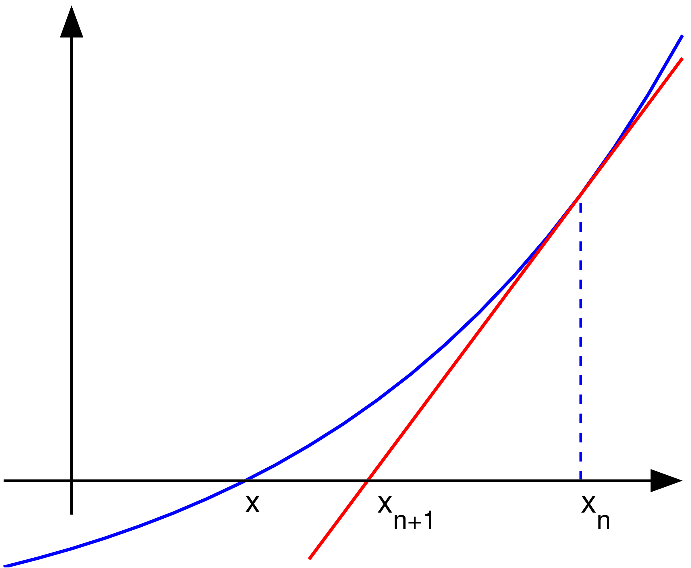
| Description | Uploader graphed this with en:MATLAB (Illustration of en:Newton's method) | ||
| Date | 22 November 2004 (first version); 2004-11-23 (last version) | ||
| Source | Transferred from en.wikipedia to Commons. | ||
| Author | Olegalexandrov at English Wikipedia | ||
| PNG development | This diagram was created with MATLAB. | ||
| Source code | MATLAB code
|
Licensing
| This work has been released into the public domain by its author, Olegalexandrov at English Wikipedia. This applies worldwide. In some countries this may not be legally possible; if so: Olegalexandrov grants anyone the right to use this work for any purpose, without any conditions, unless such conditions are required by law. |
Original upload log
The original description page was here. All following user names refer to en.wikipedia.
- 2004-11-23 19:55 Olegalexandrov 405×340×8 (14290 bytes) Scaled down the picture of Newton's method
- 2004-11-22 21:34 Olegalexandrov 509×406×8 (16510 bytes) I graphed this with Matlab (Illustration of Newton's method) {{PD}}
File history
Click on a date/time to view the file as it appeared at that time.
| Date/Time | Thumbnail | Dimensions | User | Comment | |
|---|---|---|---|---|---|
| current | 03:23, 25 May 2007 | | 2,406 × 1,978 (55 KB) | Oleg Alexandrov | {{Information |Description=Uploader graphed this with en:MATLAB (Illustration of en:Newton's method) ==Source code== <pre> <nowiki> % illustration of Newton's method for finding a zero of a function function main () a=-1; b=1; % interva |
| 23:11, 12 June 2005 |  | 405 × 340 (6 KB) | <bdi>Everlong</bdi> | optimized for smaller file size | |
| 23:06, 17 January 2005 |  | 405 × 340 (14 KB) | <bdi>Andreas Ipp~commonswiki</bdi> | {{PD}}: Original author graphed this with MATLAB (Illustration of Newton's method), from Wikipedia. |
File usage
The following pages on the English Wikipedia use this file (pages on other projects are not listed):
Global file usage
The following other wikis use this file:
- Usage on fa.wikipedia.org
- Usage on fr.wikipedia.org