Probability distribution fitting

Probability distribution fitting or simply distribution fitting is the fitting of a probability distribution to a series of data concerning the repeated measurement of a variable phenomenon. The aim of distribution fitting is to predict the probability or to forecast the frequency of occurrence of the magnitude of the phenomenon in a certain interval.

There are many probability distributions (see list of probability distributions) of which some can be fitted more closely to the observed frequency of the data than others, depending on the characteristics of the phenomenon and of the distribution. The distribution giving a close fit is supposed to lead to good predictions. In distribution fitting, therefore, one needs to select a distribution that suits the data well.

Selection of distribution

The selection of the appropriate distribution depends on the presence or absence of symmetry of the data set with respect to the central tendency.

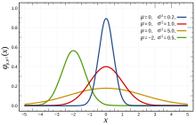
Symmetrical distributions

When the data are symmetrically distributed around the mean while the frequency of occurrence of data farther away from the mean diminishes, one may for example select the normal distribution, the logistic distribution, or the Student's t-distribution. The first two are very similar, while the last, with one degree of freedom, has "heavier tails" meaning that the values farther away from the mean occur relatively more often (i.e. the kurtosis is higher). The Cauchy distribution is also symmetric.

Skew distributions to the right

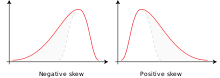
When the larger values tend to be farther away from the mean than the smaller values, one has a skew distribution to the right (i.e. there is positive skewness), one may for example select the log-normal distribution (i.e. the log values of the data are normally distributed), the log-logistic distribution (i.e. the log values of the data follow a logistic distribution), the Gumbel distribution, the exponential distribution, the Pareto distribution, the Weibull distribution, the Burr distribution, or the Fréchet distribution. The last four distributions are bounded to the left.

Skew distributions to the left

When the smaller values tend to be farther away from the mean than the larger values, one has a skew distribution to the left (i.e. there is negative skewness), one may for example select the square-normal distribution (i.e. the normal distribution applied to the square of the data values),^[1] the inverted (mirrored) Gumbel distribution,^[1] the Dagum distribution (mirrored Burr distribution), or the Gompertz distribution, which is bounded to the left.

Techniques of fitting

The following techniques of distribution fitting exist:^[2]

• Parametric methods, by which the parameters of the distribution are calculated from the data series.^[3] The parametric methods are:
  • Method of moments
  • Maximum spacing estimation
  • Method of L-moments^[4]
  • Maximum likelihood method^[5]

For example, the parameter ${\displaystyle \mu }$ (the expectation) can be estimated by the mean of the data and the parameter ${\displaystyle \sigma ^{2}}$ (the variance) can be estimated from the standard deviation of the data. The mean is found as ${\textstyle m=\sum {X}/n}$, where ${\displaystyle X}$ is the data value and ${\displaystyle n}$ the number of data, while the standard deviation is calculated as ${\textstyle s={\sqrt {{\frac {1}{n-1}}\sum {(X-m)^{2}}}}}$. With these parameters many distributions, e.g. the normal distribution, are completely defined.

• Plotting position plus Regression analysis, using a transformation of the cumulative distribution function so that a linear relation is found between the cumulative probability and the values of the data, which may also need to be transformed, depending on the selected probability distribution. In this method the cumulative probability needs to be estimated by the plotting position^[6]

For example, the cumulative Gumbel distribution can be linearized to ${\displaystyle Y=aX+b}$, where ${\displaystyle X}$ is the data variable and ${\displaystyle Y=-\ln(-\ln P)}$, with ${\displaystyle P}$ being the cumulative probability, i.e. the probability that the data value is less than ${\displaystyle X}$. Thus, using the plotting position for ${\displaystyle P}$, one finds the parameters ${\displaystyle a}$ and ${\displaystyle b}$ from a linear regression of ${\displaystyle Y}$ on ${\displaystyle X}$, and the Gumbel distribution is fully defined.

Generalization of distributions

It is customary to transform data logarithmically to fit symmetrical distributions (like the normal and logistic) to data obeying a distribution that is positively skewed (i.e. skew to the right, with mean > mode, and with a right hand tail that is longer than the left hand tail), see lognormal distribution and the loglogistic distribution. A similar effect can be achieved by taking the square root of the data.

To fit a symmetrical distribution to data obeying a negatively skewed distribution (i.e. skewed to the left, with mean < mode, and with a right hand tail this is shorter than the left hand tail) one could use the squared values of the data to accomplish the fit.

More generally one can raise the data to a power p in order to fit symmetrical distributions to data obeying a distribution of any skewness, whereby p < 1 when the skewness is positive and p > 1 when the skewness is negative. The optimal value of p is to be found by a numerical method. The numerical method may consist of assuming a range of p values, then applying the distribution fitting procedure repeatedly for all the assumed p values, and finally selecting the value of p for which the sum of squares of deviations of calculated probabilities from measured frequencies (chi squared) is minimum, as is done in CumFreq.

The generalization enhances the flexibility of probability distributions and increases their applicability in distribution fitting.^[6]

The versatility of generalization makes it possible, for example, to fit approximately normally distributed data sets to a large number of different probability distributions,^[7] while negatively skewed distributions can be fitted to square normal and mirrored Gumbel distributions.^[8]

Inversion of skewness

Skewed distributions can be inverted (or mirrored) by replacing in the mathematical expression of the cumulative distribution function (F) by its complement: F'=1-F, obtaining the complementary distribution function (also called survival function) that gives a mirror image. In this manner, a distribution that is skewed to the right is transformed into a distribution that is skewed to the left and vice versa.

Example. The F-expression of the positively skewed Gumbel distribution is: F=exp[-exp{-(X-u)/0.78s}], where u is the mode (i.e. the value occurring most frequently) and s is the standard deviation. The Gumbel distribution can be transformed using F'=1-exp[-exp{-(x-u)/0.78s}] . This transformation yields the inverse, mirrored, or complementary Gumbel distribution that may fit a data series obeying a negatively skewed distribution.

The technique of skewness inversion increases the number of probability distributions available for distribution fitting and enlarges the distribution fitting opportunities.

Shifting of distributions

Some probability distributions, like the exponential, do not support negative data values (X). Yet, when negative data are present, such distributions can still be used replacing X by Y=X-Xm, where Xm is the minimum value of X. This replacement represents a shift of the probability distribution in positive direction, i.e. to the right, because Xm is negative. After completing the distribution fitting of Y, the corresponding X-values are found from X=Y+Xm, which represents a back-shift of the distribution in negative direction, i.e. to the left.
The technique of distribution shifting augments the chance to find a properly fitting probability distribution.

Composite distributions

The option exists to use two different probability distributions, one for the lower data range, and one for the higher like for example the Laplace distribution. The ranges are separated by a break-point. The use of such composite (discontinuous) probability distributions can be opportune when the data of the phenomenon studied were obtained under two sets different conditions.^[6]

Uncertainty of prediction

Predictions of occurrence based on fitted probability distributions are subject to uncertainty, which arises from the following conditions:

• The true probability distribution of events may deviate from the fitted distribution, as the observed data series may not be totally representative of the real probability of occurrence of the phenomenon due to random error
• The occurrence of events in another situation or in the future may deviate from the fitted distribution as this occurrence can also be subject to random error
• A change of environmental conditions may cause a change in the probability of occurrence of the phenomenon

An estimate of the uncertainty in the first and second case can be obtained with the binomial probability distribution using for example the probability of exceedance Pe (i.e. the chance that the event X is larger than a reference value Xr of X) and the probability of non-exceedance Pn (i.e. the chance that the event X is smaller than or equal to the reference value Xr, this is also called cumulative probability). In this case there are only two possibilities: either there is exceedance or there is non-exceedance. This duality is the reason that the binomial distribution is applicable.

With the binomial distribution one can obtain a prediction interval. Such an interval also estimates the risk of failure, i.e. the chance that the predicted event still remains outside the confidence interval. The confidence or risk analysis may include the return period T=1/Pe as is done in hydrology.

Variance of Bayesian fitted probability functions

A Bayesian approach can be used for fitting a model ${\displaystyle P(x|\theta )}$ having a prior distribution ${\displaystyle P(\theta )}$ for the parameter ${\displaystyle \theta }$. When one has samples ${\displaystyle X}$ that are independently drawn from the underlying distribution then one can derive the so-called posterior distribution ${\displaystyle P(\theta |X)}$. This posterior can be used to update the probability mass function for a new sample ${\displaystyle x}$ given the observations ${\displaystyle X}$, one obtains

${\displaystyle P_{\theta }(x|X):=\int d\theta \ P(x|\theta )\ P(\theta |X)}$.

The variance of the newly obtained probability mass function can also be determined. The variance for a Bayesian probability mass function can be defined as

${\displaystyle \sigma _{P_{\theta }(x|X)}^{2}:=\int d\theta \ \left[P(x|\theta )-P_{\theta }(x|X)\right]^{2}\ P(\theta |X)}$.

This expression for the variance can be substantially simplified (assuming independently drawn samples). Defining the "self probability mass function" as

${\displaystyle P_{\theta }(x|\left\{X,x\right\})=\int d\theta \ P(x|\theta )\ P(\theta |\left\{X,x\right\})}$,

one obtains for the variance ^[12]

${\displaystyle \sigma _{P_{\theta }(x|X)}^{2}=P_{\theta }(x|X)\left[P_{\theta }(x|\left\{X,x\right\})-P_{\theta }(x|X)\right]}$.

The expression for variance involves an additional fit that includes the sample ${\displaystyle x}$ of interest.

Goodness of fit

By ranking the goodness of fit of various distributions one can get an impression of which distribution is acceptable and which is not.

Histogram and density function

From the cumulative distribution function (CDF) one can derive a histogram and the probability density function (PDF).

See also

• Curve fitting
• Density estimation
• Mixture distribution
• Product distribution

References

This page was last edited on 24 February 2024, at 23:02

References

- ^ a b Left (negatively) skewed frequency histograms can be fitted to square Normal or mirrored Gumbel probability functions. On line: [1]
- ^ Frequency and Regression Analysis. Chapter 6 in: H.P.Ritzema (ed., 1994), Drainage Principles and Applications, Publ. 16, pp. 175–224, International Institute for Land Reclamation and Improvement (ILRI), Wageningen, The Netherlands. ISBN 9070754339. Free download from the webpage [2] under nr. 12, or directly as PDF : [3]
- ^ H. Cramér, "Mathematical methods of statistics", Princeton Univ. Press (1946)
- ^ Hosking, J.R.M. (1990). "L-moments: analysis and estimation of distributions using linear combinations of order statistics". Journal of the Royal Statistical Society, Series B. 52 (1): 105–124. JSTOR 2345653.
- ^ Aldrich, John (1997). "R. A. Fisher and the making of maximum likelihood 1912–1922". Statistical Science. 12 (3): 162–176. doi:10.1214/ss/1030037906. MR 1617519.
- ^ a b c Software for Generalized and Composite Probability Distributions. International Journal of Mathematical and Computational Methods, 4, 1-9 [4] or [5]
- ^ Example of an approximately normally distributed data set to which a large number of different probability distributions can be fitted, [6]
- ^ Left (negatively) skewed frequency histograms can be fitted to square normal or mirrored Gumbel probability functions. [7]
- ^ Intro to composite probability distributions
- ^ Frequency predictions and their binomial confidence limits. In: International Commission on Irrigation and Drainage, Special Technical Session: Economic Aspects of Flood Control and non-Structural Measures, Dubrovnik, Yugoslavia, 1988. On line
- ^ Benson, M.A. 1960. Characteristics of frequency curves based on a theoretical 1000 year record. In: T.Dalrymple (Ed.), Flood frequency analysis. U.S. Geological Survey Water Supply Paper, 1543-A, pp. 51-71.
- ^ Pijlman; Linnartz (2023). "Variance of Likelihood of data". SITB 2023 Proceedings: 34.
- ^ Software for probability distribution fitting