


In mathematics (in particular, functional analysis), convolution is a mathematical operation on two functions ( and ) that produces a third function (). The term convolution refers to both the result function and to the process of computing it. It is defined as the integral of the product of the two functions after one is reflected about the y-axis and shifted. The integral is evaluated for all values of shift, producing the convolution function. The choice of which function is reflected and shifted before the integral does not change the integral result (see commutativity). Graphically, it expresses how the 'shape' of one function is modified by the other.


Some features of convolution are similar to cross-correlation: for real-valued functions, of a continuous or discrete variable, convolution () differs from cross-correlation () only in that either or is reflected about the y-axis in convolution; thus it is a cross-correlation of and , or and .[A] For complex-valued functions, the cross-correlation operator is the adjoint of the convolution operator.


Convolution has applications that include probability, statistics, acoustics, spectroscopy, signal processing and image processing, geophysics, engineering, physics, computer vision and differential equations.[1]
The convolution can be defined for functions on Euclidean space and other groups (as algebraic structures).[citation needed] For example, periodic functions, such as the discrete-time Fourier transform, can be defined on a circle and convolved by periodic convolution. (See row 18 at DTFT § Properties.) A discrete convolution can be defined for functions on the set of integers.
Generalizations of convolution have applications in the field of numerical analysis and numerical linear algebra, and in the design and implementation of finite impulse response filters in signal processing.[citation needed]
Computing the inverse of the convolution operation is known as deconvolution.
YouTube Encyclopedic
-
1/5Views:230 9072 349 661231 90435 48470 161
-
The Convolution of Two Functions | Definition & Properties
-
But what is a convolution?
-
Tutorial 21- What is Convolution operation in CNN?
-
How to Understand Convolution ("This is an incredible explanation")
-
Convolution integral example - graphical method
Transcription
Definition
The convolution of and is written , denoting the operator with the symbol .[B] It is defined as the integral of the product of the two functions after one is reflected about the y-axis and shifted. As such, it is a particular kind of integral transform:


An equivalent definition is (see commutativity):

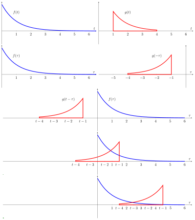
While the symbol is used above, it need not represent the time domain. At each , the convolution formula can be described as the area under the function weighted by the function shifted by the amount . As changes, the weighting function emphasizes different parts of the input function ; If is a positive value, then is equal to that slides or is shifted along the -axis toward the right (toward ) by the amount of , while if is a negative value, then is equal to that slides or is shifted toward the left (toward ) by the amount of .


For functions , supported on only (i.e., zero for negative arguments), the integration limits can be truncated, resulting in:
![{\displaystyle [0,\infty ]}](https://wikimedia.org/api/rest_v1/media/math/render/svg/52088d5605716e18068a460dec118214954a68e9)

For the multi-dimensional formulation of convolution, see domain of definition (below).
Notation
A common engineering notational convention is:[2]

which has to be interpreted carefully to avoid confusion. For instance, is equivalent to , but is in fact equivalent to .[3]


Relations with other transforms
Given two functions and with bilateral Laplace transforms (two-sided Laplace transform)


and

respectively, the convolution operation can be defined as the inverse Laplace transform of the product of and .[4][5] More precisely,


Let such that


Note that is the bilateral Laplace transform of . A similar derivation can be done using the unilateral Laplace transform (one-sided Laplace transform).

The convolution operation also describes the output (in terms of the input) of an important class of operations known as linear time-invariant (LTI). See LTI system theory for a derivation of convolution as the result of LTI constraints. In terms of the Fourier transforms of the input and output of an LTI operation, no new frequency components are created. The existing ones are only modified (amplitude and/or phase). In other words, the output transform is the pointwise product of the input transform with a third transform (known as a transfer function). See Convolution theorem for a derivation of that property of convolution. Conversely, convolution can be derived as the inverse Fourier transform of the pointwise product of two Fourier transforms.
Visual explanation
The resulting waveform (not shown here) is the convolution of functions f and g. If is a unit impulse, the result of this process is simply . Formally: |
 |
| In this example, the red-colored "pulse", is an even function so convolution is equivalent to correlation. A snapshot of this "movie" shows functions and (in blue) for some value of parameter which is arbitrarily defined as the distance along the axis from the point to the center of the red pulse. The amount of yellow is the area of the product computed by the convolution/correlation integral. The movie is created by continuously changing and recomputing the integral. The result (shown in black) is a function of but is plotted on the same axis as for convenience and comparison. | 
|
| In this depiction, could represent the response of a resistor-capacitor circuit to a narrow pulse that occurs at In other words, if the result of convolution is just But when is the wider pulse (in red), the response is a "smeared" version of It begins at because we defined as the distance from the axis to the center of the wide pulse (instead of the leading edge). | 
|


Historical developments
One of the earliest uses of the convolution integral appeared in D'Alembert's derivation of Taylor's theorem in Recherches sur différents points importants du système du monde, published in 1754.[6]
Also, an expression of the type:

is used by Sylvestre François Lacroix on page 505 of his book entitled Treatise on differences and series, which is the last of 3 volumes of the encyclopedic series: Traité du calcul différentiel et du calcul intégral, Chez Courcier, Paris, 1797–1800.[7] Soon thereafter, convolution operations appear in the works of Pierre Simon Laplace, Jean-Baptiste Joseph Fourier, Siméon Denis Poisson, and others. The term itself did not come into wide use until the 1950s or 60s. Prior to that it was sometimes known as Faltung (which means folding in German), composition product, superposition integral, and Carson's integral.[8] Yet it appears as early as 1903, though the definition is rather unfamiliar in older uses.[9][10]
The operation:

is a particular case of composition products considered by the Italian mathematician Vito Volterra in 1913.[11]
Circular convolution
When a function gT is periodic, with period T, then for functions, f, such that f ∗ gT exists, the convolution is also periodic and identical to:
![{\displaystyle (f*g_{T})(t)\equiv \int _{t_{0}}^{t_{0}+T}\left[\sum _{k=-\infty }^{\infty }f(\tau +kT)\right]g_{T}(t-\tau )\,d\tau ,}](https://wikimedia.org/api/rest_v1/media/math/render/svg/46ca67ae76bc1e6841511aa12fab10aed9cb970d)
where t0 is an arbitrary choice. The summation is called a periodic summation of the function f.
When gT is a periodic summation of another function, g, then f ∗ gT is known as a circular or cyclic convolution of f and g.
And if the periodic summation above is replaced by fT, the operation is called a periodic convolution of fT and gT.
Discrete convolution

For complex-valued functions f, g defined on the set Z of integers, the discrete convolution of f and g is given by:[12]
![{\displaystyle (f*g)[n]=\sum _{m=-\infty }^{\infty }f[m]g[n-m],}](https://wikimedia.org/api/rest_v1/media/math/render/svg/ea98dff26dac2459282e10b7c7e4f5e5b6c91dad)
or equivalently (see commutativity) by:
![{\displaystyle (f*g)[n]=\sum _{m=-\infty }^{\infty }f[n-m]g[m].}](https://wikimedia.org/api/rest_v1/media/math/render/svg/c98a8db58f6ced1a80968fe0f2c99a7a81e782f0)
The convolution of two finite sequences is defined by extending the sequences to finitely supported functions on the set of integers. When the sequences are the coefficients of two polynomials, then the coefficients of the ordinary product of the two polynomials are the convolution of the original two sequences. This is known as the Cauchy product of the coefficients of the sequences.
Thus when g has finite support in the set (representing, for instance, a finite impulse response), a finite summation may be used:[13]

![{\displaystyle (f*g)[n]=\sum _{m=-M}^{M}f[n-m]g[m].}](https://wikimedia.org/api/rest_v1/media/math/render/svg/fddacde29cbcb3c6fca263493335c31a4d2ebce2)
Circular discrete convolution
When a function gN is periodic, with period N, then for functions, f, such that f∗gN exists, the convolution is also periodic and identical to:
![{\displaystyle (f*g_{N})[n]\equiv \sum _{m=0}^{N-1}\left(\sum _{k=-\infty }^{\infty }{f}[m+kN]\right)g_{N}[n-m].}](https://wikimedia.org/api/rest_v1/media/math/render/svg/a89c13781ae07c2cfdf62cee30ca8139e1fea632)
The summation on k is called a periodic summation of the function f.
If gN is a periodic summation of another function, g, then f∗gN is known as a circular convolution of f and g.
When the non-zero durations of both f and g are limited to the interval [0, N − 1], f∗gN reduces to these common forms:
-
(Eq.1)
![{\displaystyle {\begin{aligned}\left(f*g_{N}\right)[n]&=\sum _{m=0}^{N-1}f[m]g_{N}[n-m]\\&=\sum _{m=0}^{n}f[m]g[n-m]+\sum _{m=n+1}^{N-1}f[m]g[N+n-m]\\[2pt]&=\sum _{m=0}^{N-1}f[m]g[(n-m)_{\bmod {N}}]\\[2pt]&\triangleq \left(f*_{N}g\right)[n]\end{aligned}}}](https://wikimedia.org/api/rest_v1/media/math/render/svg/2ea93687815cb3c2fe0ef1acee64c01b50f9e421)
The notation for cyclic convolution denotes convolution over the cyclic group of integers modulo N.

Circular convolution arises most often in the context of fast convolution with a fast Fourier transform (FFT) algorithm.
Fast convolution algorithms
In many situations, discrete convolutions can be converted to circular convolutions so that fast transforms with a convolution property can be used to implement the computation. For example, convolution of digit sequences is the kernel operation in multiplication of multi-digit numbers, which can therefore be efficiently implemented with transform techniques (Knuth 1997, §4.3.3.C; von zur Gathen & Gerhard 2003, §8.2).
Eq.1 requires N arithmetic operations per output value and N2 operations for N outputs. That can be significantly reduced with any of several fast algorithms. Digital signal processing and other applications typically use fast convolution algorithms to reduce the cost of the convolution to O(N log N) complexity.
The most common fast convolution algorithms use fast Fourier transform (FFT) algorithms via the circular convolution theorem. Specifically, the circular convolution of two finite-length sequences is found by taking an FFT of each sequence, multiplying pointwise, and then performing an inverse FFT. Convolutions of the type defined above are then efficiently implemented using that technique in conjunction with zero-extension and/or discarding portions of the output. Other fast convolution algorithms, such as the Schönhage–Strassen algorithm or the Mersenne transform,[14] use fast Fourier transforms in other rings. The Winograd method is used as an alternative to the FFT.[15] It significantly speeds up 1D,[16] 2D,[17] and 3D[18] convolution.
If one sequence is much longer than the other, zero-extension of the shorter sequence and fast circular convolution is not the most computationally efficient method available.[19] Instead, decomposing the longer sequence into blocks and convolving each block allows for faster algorithms such as the overlap–save method and overlap–add method.[20] A hybrid convolution method that combines block and FIR algorithms allows for a zero input-output latency that is useful for real-time convolution computations.[21]
Domain of definition
The convolution of two complex-valued functions on Rd is itself a complex-valued function on Rd, defined by:

and is well-defined only if f and g decay sufficiently rapidly at infinity in order for the integral to exist. Conditions for the existence of the convolution may be tricky, since a blow-up in g at infinity can be easily offset by sufficiently rapid decay in f. The question of existence thus may involve different conditions on f and g:
Compactly supported functions
If f and g are compactly supported continuous functions, then their convolution exists, and is also compactly supported and continuous (Hörmander 1983, Chapter 1). More generally, if either function (say f) is compactly supported and the other is locally integrable, then the convolution f∗g is well-defined and continuous.
Convolution of f and g is also well defined when both functions are locally square integrable on R and supported on an interval of the form [a, +∞) (or both supported on [−∞, a]).
Integrable functions
The convolution of f and g exists if f and g are both Lebesgue integrable functions in L1(Rd), and in this case f∗g is also integrable (Stein & Weiss 1971, Theorem 1.3). This is a consequence of Tonelli's theorem. This is also true for functions in L1, under the discrete convolution, or more generally for the convolution on any group.
Likewise, if f ∈ L1(Rd) and g ∈ Lp(Rd) where 1 ≤ p ≤ ∞, then f*g ∈ Lp(Rd), and

In the particular case p = 1, this shows that L1 is a Banach algebra under the convolution (and equality of the two sides holds if f and g are non-negative almost everywhere).
More generally, Young's inequality implies that the convolution is a continuous bilinear map between suitable Lp spaces. Specifically, if 1 ≤ p, q, r ≤ ∞ satisfy:

then

so that the convolution is a continuous bilinear mapping from Lp×Lq to Lr. The Young inequality for convolution is also true in other contexts (circle group, convolution on Z). The preceding inequality is not sharp on the real line: when 1 < p, q, r < ∞, there exists a constant Bp,q < 1 such that:

The optimal value of Bp,q was discovered in 1975[22] and independently in 1976,[23] see Brascamp–Lieb inequality.
A stronger estimate is true provided 1 < p, q, r < ∞:

where is the weak Lq norm. Convolution also defines a bilinear continuous map for , owing to the weak Young inequality:[24]


Functions of rapid decay
In addition to compactly supported functions and integrable functions, functions that have sufficiently rapid decay at infinity can also be convolved. An important feature of the convolution is that if f and g both decay rapidly, then f∗g also decays rapidly. In particular, if f and g are rapidly decreasing functions, then so is the convolution f∗g. Combined with the fact that convolution commutes with differentiation (see #Properties), it follows that the class of Schwartz functions is closed under convolution (Stein & Weiss 1971, Theorem 3.3).
Distributions
If f is a smooth function that is compactly supported and g is a distribution, then f∗g is a smooth function defined by

More generally, it is possible to extend the definition of the convolution in a unique way with the same as f above, so that the associative law


remains valid in the case where f is a distribution, and g a compactly supported distribution (Hörmander 1983, §4.2).
Measures
The convolution of any two Borel measures μ and ν of bounded variation is the measure defined by (Rudin 1962)


In particular,

where is a measurable set and is the indicator function of .


This agrees with the convolution defined above when μ and ν are regarded as distributions, as well as the convolution of L1 functions when μ and ν are absolutely continuous with respect to the Lebesgue measure.
The convolution of measures also satisfies the following version of Young's inequality

where the norm is the total variation of a measure. Because the space of measures of bounded variation is a Banach space, convolution of measures can be treated with standard methods of functional analysis that may not apply for the convolution of distributions.
Properties
Algebraic properties
The convolution defines a product on the linear space of integrable functions. This product satisfies the following algebraic properties, which formally mean that the space of integrable functions with the product given by convolution is a commutative associative algebra without identity (Strichartz 1994, §3.3). Other linear spaces of functions, such as the space of continuous functions of compact support, are closed under the convolution, and so also form commutative associative algebras.
- Commutativity
- Proof: By definition:Changing the variable of integration to the result follows.


- Associativity
- Proof: This follows from using Fubini's theorem (i.e., double integrals can be evaluated as iterated integrals in either order).

- Distributivity
- Proof: This follows from linearity of the integral.

- Associativity with scalar multiplication
- for any real (or complex) number .


- Multiplicative identity
- No algebra of functions possesses an identity for the convolution. The lack of identity is typically not a major inconvenience, since most collections of functions on which the convolution is performed can be convolved with a delta distribution (a unitary impulse, centered at zero) or, at the very least (as is the case of L1) admit approximations to the identity. The linear space of compactly supported distributions does, however, admit an identity under the convolution. Specifically, where δ is the delta distribution.

- Inverse element
- Some distributions S have an inverse element S−1 for the convolution which then must satisfy from which an explicit formula for S−1 may be obtained.The set of invertible distributions forms an abelian group under the convolution.

- Complex conjugation

- Relationship with differentiation
- Proof:


- Relationship with integration
- If and then


Integration
If f and g are integrable functions, then the integral of their convolution on the whole space is simply obtained as the product of their integrals:[25]

This follows from Fubini's theorem. The same result holds if f and g are only assumed to be nonnegative measurable functions, by Tonelli's theorem.
Differentiation
In the one-variable case,

where is the derivative. More generally, in the case of functions of several variables, an analogous formula holds with the partial derivative:


A particular consequence of this is that the convolution can be viewed as a "smoothing" operation: the convolution of f and g is differentiable as many times as f and g are in total.
These identities hold under the precise condition that f and g are absolutely integrable and at least one of them has an absolutely integrable (L1) weak derivative, as a consequence of Young's convolution inequality. For instance, when f is continuously differentiable with compact support, and g is an arbitrary locally integrable function,

These identities also hold much more broadly in the sense of tempered distributions if one of f or g is a rapidly decreasing tempered distribution, a compactly supported tempered distribution or a Schwartz function and the other is a tempered distribution. On the other hand, two positive integrable and infinitely differentiable functions may have a nowhere continuous convolution.
In the discrete case, the difference operator D f(n) = f(n + 1) − f(n) satisfies an analogous relationship:

Convolution theorem
The convolution theorem states that[26]

where denotes the Fourier transform of .

Convolution in other types of transformations
Versions of this theorem also hold for the Laplace transform, two-sided Laplace transform, Z-transform and Mellin transform.
Convolution on matrices
If is the Fourier transform matrix, then

- ,

where is face-splitting product,[27][28][29][30][31] denotes Kronecker product, denotes Hadamard product (this result is an evolving of count sketch properties[32]).


Translational equivariance
The convolution commutes with translations, meaning that

where τxf is the translation of the function f by x defined by

If f is a Schwartz function, then τxf is the convolution with a translated Dirac delta function τxf = f ∗ τx δ. So translation invariance of the convolution of Schwartz functions is a consequence of the associativity of convolution.
Furthermore, under certain conditions, convolution is the most general translation invariant operation. Informally speaking, the following holds
- Suppose that S is a bounded linear operator acting on functions which commutes with translations: S(τxf) = τx(Sf) for all x. Then S is given as convolution with a function (or distribution) gS; that is Sf = gS ∗ f.
Thus some translation invariant operations can be represented as convolution. Convolutions play an important role in the study of time-invariant systems, and especially LTI system theory. The representing function gS is the impulse response of the transformation S.
A more precise version of the theorem quoted above requires specifying the class of functions on which the convolution is defined, and also requires assuming in addition that S must be a continuous linear operator with respect to the appropriate topology. It is known, for instance, that every continuous translation invariant continuous linear operator on L1 is the convolution with a finite Borel measure. More generally, every continuous translation invariant continuous linear operator on Lp for 1 ≤ p < ∞ is the convolution with a tempered distribution whose Fourier transform is bounded. To wit, they are all given by bounded Fourier multipliers.
Convolutions on groups
If G is a suitable group endowed with a measure λ, and if f and g are real or complex valued integrable functions on G, then we can define their convolution by

It is not commutative in general. In typical cases of interest G is a locally compact Hausdorff topological group and λ is a (left-) Haar measure. In that case, unless G is unimodular, the convolution defined in this way is not the same as . The preference of one over the other is made so that convolution with a fixed function g commutes with left translation in the group:


Furthermore, the convention is also required for consistency with the definition of the convolution of measures given below. However, with a right instead of a left Haar measure, the latter integral is preferred over the former.
On locally compact abelian groups, a version of the convolution theorem holds: the Fourier transform of a convolution is the pointwise product of the Fourier transforms. The circle group T with the Lebesgue measure is an immediate example. For a fixed g in L1(T), we have the following familiar operator acting on the Hilbert space L2(T):

The operator T is compact. A direct calculation shows that its adjoint T* is convolution with

By the commutativity property cited above, T is normal: T* T = TT* . Also, T commutes with the translation operators. Consider the family S of operators consisting of all such convolutions and the translation operators. Then S is a commuting family of normal operators. According to spectral theory, there exists an orthonormal basis {hk} that simultaneously diagonalizes S. This characterizes convolutions on the circle. Specifically, we have

which are precisely the characters of T. Each convolution is a compact multiplication operator in this basis. This can be viewed as a version of the convolution theorem discussed above.
A discrete example is a finite cyclic group of order n. Convolution operators are here represented by circulant matrices, and can be diagonalized by the discrete Fourier transform.
A similar result holds for compact groups (not necessarily abelian): the matrix coefficients of finite-dimensional unitary representations form an orthonormal basis in L2 by the Peter–Weyl theorem, and an analog of the convolution theorem continues to hold, along with many other aspects of harmonic analysis that depend on the Fourier transform.
Convolution of measures
Let G be a (multiplicatively written) topological group. If μ and ν are finite Borel measures on G, then their convolution μ∗ν is defined as the pushforward measure of the group action and can be written as

for each measurable subset E of G. The convolution is also a finite measure, whose total variation satisfies

In the case when G is locally compact with (left-)Haar measure λ, and μ and ν are absolutely continuous with respect to a λ, so that each has a density function, then the convolution μ∗ν is also absolutely continuous, and its density function is just the convolution of the two separate density functions.
If μ and ν are probability measures on the topological group (R,+), then the convolution μ∗ν is the probability distribution of the sum X + Y of two independent random variables X and Y whose respective distributions are μ and ν.
Infimal convolution
In convex analysis, the infimal convolution of proper (not identically ) convex functions on is defined by:[33]


Bialgebras
Let (X, Δ, ∇, ε, η) be a bialgebra with comultiplication Δ, multiplication ∇, unit η, and counit ε. The convolution is a product defined on the endomorphism algebra End(X) as follows. Let φ, ψ ∈ End(X), that is, φ, ψ: X → X are functions that respect all algebraic structure of X, then the convolution φ∗ψ is defined as the composition

The convolution appears notably in the definition of Hopf algebras (Kassel 1995, §III.3). A bialgebra is a Hopf algebra if and only if it has an antipode: an endomorphism S such that

Applications

Convolution and related operations are found in many applications in science, engineering and mathematics.
- Convolutional neural networks apply multiple cascaded convolution kernels with applications in machine vision and artificial intelligence.[34][35] Though these are actually cross-correlations rather than convolutions in most cases.[36]
- In non-neural-network-based image processing
- In digital image processing convolutional filtering plays an important role in many important algorithms in edge detection and related processes (see Kernel (image processing))
- In optics, an out-of-focus photograph is a convolution of the sharp image with a lens function. The photographic term for this is bokeh.
- In image processing applications such as adding blurring.
- In digital data processing
- In analytical chemistry, Savitzky–Golay smoothing filters are used for the analysis of spectroscopic data. They can improve signal-to-noise ratio with minimal distortion of the spectra
- In statistics, a weighted moving average is a convolution.
- In acoustics, reverberation is the convolution of the original sound with echoes from objects surrounding the sound source.
- In digital signal processing, convolution is used to map the impulse response of a real room on a digital audio signal.
- In electronic music convolution is the imposition of a spectral or rhythmic structure on a sound. Often this envelope or structure is taken from another sound. The convolution of two signals is the filtering of one through the other.[37]
- In electrical engineering, the convolution of one function (the input signal) with a second function (the impulse response) gives the output of a linear time-invariant system (LTI). At any given moment, the output is an accumulated effect of all the prior values of the input function, with the most recent values typically having the most influence (expressed as a multiplicative factor). The impulse response function provides that factor as a function of the elapsed time since each input value occurred.
- In physics, wherever there is a linear system with a "superposition principle", a convolution operation makes an appearance. For instance, in spectroscopy line broadening due to the Doppler effect on its own gives a Gaussian spectral line shape and collision broadening alone gives a Lorentzian line shape. When both effects are operative, the line shape is a convolution of Gaussian and Lorentzian, a Voigt function.
- In time-resolved fluorescence spectroscopy, the excitation signal can be treated as a chain of delta pulses, and the measured fluorescence is a sum of exponential decays from each delta pulse.
- In computational fluid dynamics, the large eddy simulation (LES) turbulence model uses the convolution operation to lower the range of length scales necessary in computation thereby reducing computational cost.
- In probability theory, the probability distribution of the sum of two independent random variables is the convolution of their individual distributions.
- In kernel density estimation, a distribution is estimated from sample points by convolution with a kernel, such as an isotropic Gaussian.[38]
- In radiotherapy treatment planning systems, most part of all modern codes of calculation applies a convolution-superposition algorithm.[clarification needed]
- In structural reliability, the reliability index can be defined based on the convolution theorem.
- The definition of reliability index for limit state functions with nonnormal distributions can be established corresponding to the joint distribution function. In fact, the joint distribution function can be obtained using the convolution theory.[39]
- In Smoothed-particle hydrodynamics, simulations of fluid dynamics are calculated using particles, each with surrounding kernels. For any given particle , some physical quantity is calculated as a convolution of with a weighting function, where denotes the neighbors of particle : those that are located within its kernel. The convolution is approximated as a summation over each neighbor.[40]
- In Fractional calculus convolution is instrumental in various definitions of fractional integral and fractional derivative.


See also
- Analog signal processing
- Circulant matrix
- Convolution for optical broad-beam responses in scattering media
- Convolution power
- Convolution quotient
- Dirichlet convolution
- Generalized signal averaging
- List of convolutions of probability distributions
- LTI system theory#Impulse response and convolution
- Multidimensional discrete convolution
- Scaled correlation
- Titchmarsh convolution theorem
- Toeplitz matrix (convolutions can be considered a Toeplitz matrix operation where each row is a shifted copy of the convolution kernel)
- Wavelet transform
Notes
- ^ Reasons for the reflection include:
- It is necessary to implement the equivalent of the pointwise product of the Fourier transforms of and .
- When the convolution is viewed as a moving weighted average, the weighting function, , is often specified in terms of another function, , called the impulse response of a linear time-invariant system.
- ^ The symbol U+2217 ∗ ASTERISK OPERATOR is different than U+002A * ASTERISK, which is often used to denote complex conjugation. See Asterisk § Mathematical typography.
References
- ^ Bahri, Mawardi; Ashino, Ryuichi; Vaillancourt, Rémi (2013). "Convolution Theorems for Quaternion Fourier Transform: Properties and Applications" (PDF). Abstract and Applied Analysis. 2013: 1–10. doi:10.1155/2013/162769. Archived (PDF) from the original on 2020-10-21. Retrieved 2022-11-11.
- ^ Smith, Stephen W (1997). "13.Convolution". The Scientist and Engineer's Guide to Digital Signal Processing (1 ed.). California Technical Publishing. ISBN 0-9660176-3-3. Retrieved 22 April 2016.
- ^ Irwin, J. David (1997). "4.3". The Industrial Electronics Handbook (1 ed.). Boca Raton, FL: CRC Press. p. 75. ISBN 0-8493-8343-9.
- ^ Differential Equations (Spring 2010), MIT 18.03. "Lecture 21: Convolution Formula". MIT Open Courseware. MIT. Retrieved 22 December 2021.
{{cite web}}: CS1 maint: numeric names: authors list (link) - ^ "18.03SC Differential Equations Fall 2011" (PDF). Green's Formula, Laplace Transform of Convolution. Archived (PDF) from the original on 2015-09-06.
- ^ Dominguez-Torres, p 2
- ^ Dominguez-Torres, p 4
- ^ R. N. Bracewell (2005), "Early work on imaging theory in radio astronomy", in W. T. Sullivan (ed.), The Early Years of Radio Astronomy: Reflections Fifty Years After Jansky's Discovery, Cambridge University Press, p. 172, ISBN 978-0-521-61602-7
- ^ John Hilton Grace and Alfred Young (1903), The algebra of invariants, Cambridge University Press, p. 40
- ^ Leonard Eugene Dickson (1914), Algebraic invariants, J. Wiley, p. 85
- ^ According to [Lothar von Wolfersdorf (2000), "Einige Klassen quadratischer Integralgleichungen", Sitzungsberichte der Sächsischen Akademie der Wissenschaften zu Leipzig, Mathematisch-naturwissenschaftliche Klasse, volume 128, number 2, 6–7], the source is Volterra, Vito (1913), "Leçons sur les fonctions de linges". Gauthier-Villars, Paris 1913.
- ^ Damelin & Miller 2011, p. 219
- ^ Press, William H.; Flannery, Brian P.; Teukolsky, Saul A.; Vetterling, William T. (1989). Numerical Recipes in Pascal. Cambridge University Press. p. 450. ISBN 0-521-37516-9.
- ^ Rader, C.M. (December 1972). "Discrete Convolutions via Mersenne Transforms". IEEE Transactions on Computers. 21 (12): 1269–1273. doi:10.1109/T-C.1972.223497. S2CID 1939809.
- ^ Winograd, Shmuel (January 1980). Arithmetic Complexity of Computations. Society for Industrial and Applied Mathematics. doi:10.1137/1.9781611970364. ISBN 978-0-89871-163-9.
- ^ Lyakhov, P. A.; Nagornov, N. N.; Semyonova, N. F.; Abdulsalyamova, A. S. (June 2023). "Reducing the Computational Complexity of Image Processing Using Wavelet Transform Based on the Winograd Method". Pattern Recognition and Image Analysis. 33 (2): 184–191. doi:10.1134/S1054661823020074. ISSN 1054-6618. S2CID 259310351.
- ^ Wu, Di; Fan, Xitian; Cao, Wei; Wang, Lingli (May 2021). "SWM: A High-Performance Sparse-Winograd Matrix Multiplication CNN Accelerator". IEEE Transactions on Very Large Scale Integration (VLSI) Systems. 29 (5): 936–949. doi:10.1109/TVLSI.2021.3060041. ISSN 1063-8210. S2CID 233433757.
- ^ Mittal, Sparsh; Vibhu (May 2021). "A survey of accelerator architectures for 3D convolution neural networks". Journal of Systems Architecture. 115: 102041. doi:10.1016/j.sysarc.2021.102041. S2CID 233917781.
- ^ Selesnick, Ivan W.; Burrus, C. Sidney (1999). "Fast Convolution and Filtering". In Madisetti, Vijay K. (ed.). Digital Signal Processing Handbook. CRC Press. p. Section 8. ISBN 978-1-4200-4563-5.
- ^ Juang, B.H. "Lecture 21: Block Convolution" (PDF). EECS at the Georgia Institute of Technology. Archived (PDF) from the original on 2004-07-29. Retrieved 17 May 2013.
- ^ Gardner, William G. (November 1994). "Efficient Convolution without Input/Output Delay" (PDF). Audio Engineering Society Convention 97. Paper 3897. Archived (PDF) from the original on 2015-04-08. Retrieved 17 May 2013.
- ^ Beckner, William (1975). "Inequalities in Fourier analysis". Annals of Mathematics. Second Series. 102 (1): 159–182. doi:10.2307/1970980. JSTOR 1970980.
- ^ Brascamp, Herm Jan; Lieb, Elliott H. (1976). "Best constants in Young's inequality, its converse, and its generalization to more than three functions". Advances in Mathematics. 20 (2): 151–173. doi:10.1016/0001-8708(76)90184-5.
- ^ Reed & Simon 1975, IX.4
- ^ Weisstein, Eric W. "Convolution". mathworld.wolfram.com. Retrieved 2021-09-22.
- ^ Weisstein, Eric W. "From MathWorld--A Wolfram Web Resource".
- ^ Slyusar, V. I. (December 27, 1996). "End products in matrices in radar applications" (PDF). Radioelectronics and Communications Systems. 41 (3): 50–53. Archived (PDF) from the original on 2013-08-11.
- ^ Slyusar, V. I. (1997-05-20). "Analytical model of the digital antenna array on a basis of face-splitting matrix products" (PDF). Proc. ICATT-97, Kyiv: 108–109. Archived (PDF) from the original on 2013-08-11.
- ^ Slyusar, V. I. (1997-09-15). "New operations of matrices product for applications of radars" (PDF). Proc. Direct and Inverse Problems of Electromagnetic and Acoustic Wave Theory (DIPED-97), Lviv.: 73–74. Archived (PDF) from the original on 2013-08-11.
- ^ Slyusar, V. I. (March 13, 1998). "A Family of Face Products of Matrices and its Properties" (PDF). Cybernetics and Systems Analysis C/C of Kibernetika I Sistemnyi Analiz.- 1999. 35 (3): 379–384. doi:10.1007/BF02733426. S2CID 119661450. Archived (PDF) from the original on 2013-08-11.
- ^ Slyusar, V. I. (2003). "Generalized face-products of matrices in models of digital antenna arrays with nonidentical channels" (PDF). Radioelectronics and Communications Systems. 46 (10): 9–17. Archived (PDF) from the original on 2013-08-11.
- ^ Ninh, Pham; Pagh, Rasmus (2013). Fast and scalable polynomial kernels via explicit feature maps. SIGKDD international conference on Knowledge discovery and data mining. Association for Computing Machinery. doi:10.1145/2487575.2487591.
- ^ R. Tyrrell Rockafellar (1970), Convex analysis, Princeton University Press
- ^ Zhang, Yingjie; Soon, Hong Geok; Ye, Dongsen; Fuh, Jerry Ying Hsi; Zhu, Kunpeng (September 2020). "Powder-Bed Fusion Process Monitoring by Machine Vision With Hybrid Convolutional Neural Networks". IEEE Transactions on Industrial Informatics. 16 (9): 5769–5779. doi:10.1109/TII.2019.2956078. ISSN 1941-0050. S2CID 213010088.
- ^ Chervyakov, N.I.; Lyakhov, P.A.; Deryabin, M.A.; Nagornov, N.N.; Valueva, M.V.; Valuev, G.V. (September 2020). "Residue Number System-Based Solution for Reducing the Hardware Cost of a Convolutional Neural Network". Neurocomputing. 407: 439–453. doi:10.1016/j.neucom.2020.04.018. S2CID 219470398.
Convolutional neural networks represent deep learning architectures that are currently used in a wide range of applications, including computer vision, speech recognition, time series analysis in finance, and many others.
- ^ Atlas, Homma, and Marks. "An Artificial Neural Network for Spatio-Temporal Bipolar Patterns: Application to Phoneme Classification" (PDF). Neural Information Processing Systems (NIPS 1987). 1. Archived (PDF) from the original on 2021-04-14.
{{cite journal}}: CS1 maint: multiple names: authors list (link) - ^ Zölzer, Udo, ed. (2002). DAFX:Digital Audio Effects, p.48–49. ISBN 0471490784.
- ^ Diggle 1985.
- ^ Ghasemi & Nowak 2017.
- ^ Monaghan, J. J. (1992). "Smoothed particle hydrodynamics". Annual Review of Astronomy and Astrophysics. 30: 543–547. Bibcode:1992ARA&A..30..543M. doi:10.1146/annurev.aa.30.090192.002551. Retrieved 16 February 2021.
Further reading
- Bracewell, R. (1986), The Fourier Transform and Its Applications (2nd ed.), McGraw–Hill, ISBN 0-07-116043-4.
- Damelin, S.; Miller, W. (2011), The Mathematics of Signal Processing, Cambridge University Press, ISBN 978-1107601048
- Diggle, P. J. (1985), "A kernel method for smoothing point process data", Journal of the Royal Statistical Society, Series C, 34 (2): 138–147, doi:10.2307/2347366, JSTOR 2347366, S2CID 116746157
- Dominguez-Torres, Alejandro (Nov 2, 2010). "Origin and history of convolution". 41 pgs. https://slideshare.net/Alexdfar/origin-adn-history-of-convolution. Cranfield, Bedford MK43 OAL, UK. Retrieved Mar 13, 2013.
- Ghasemi, S. Hooman; Nowak, Andrzej S. (2017), "Reliability Index for Non-normal Distributions of Limit State Functions", Structural Engineering and Mechanics, 62 (3): 365–372, doi:10.12989/sem.2017.62.3.365
- Grinshpan, A. Z. (2017), "An inequality for multiple convolutions with respect to Dirichlet probability measure", Advances in Applied Mathematics, 82 (1): 102–119, doi:10.1016/j.aam.2016.08.001
- Hewitt, Edwin; Ross, Kenneth A. (1979), Abstract harmonic analysis. Vol. I, Grundlehren der Mathematischen Wissenschaften [Fundamental Principles of Mathematical Sciences], vol. 115 (2nd ed.), Berlin, New York: Springer-Verlag, ISBN 978-3-540-09434-0, MR 0551496.
- Hewitt, Edwin; Ross, Kenneth A. (1970), Abstract harmonic analysis. Vol. II: Structure and analysis for compact groups. Analysis on locally compact Abelian groups, Die Grundlehren der mathematischen Wissenschaften, Band 152, Berlin, New York: Springer-Verlag, MR 0262773.
- Hörmander, L. (1983), The analysis of linear partial differential operators I, Grundl. Math. Wissenschaft., vol. 256, Springer, doi:10.1007/978-3-642-96750-4, ISBN 3-540-12104-8, MR 0717035.
- Kassel, Christian (1995), Quantum groups, Graduate Texts in Mathematics, vol. 155, Berlin, New York: Springer-Verlag, doi:10.1007/978-1-4612-0783-2, ISBN 978-0-387-94370-1, MR 1321145.
- Knuth, Donald (1997), Seminumerical Algorithms (3rd. ed.), Reading, Massachusetts: Addison–Wesley, ISBN 0-201-89684-2.
- Narici, Lawrence; Beckenstein, Edward (2011). Topological Vector Spaces. Pure and applied mathematics (Second ed.). Boca Raton, FL: CRC Press. ISBN 978-1584888666. OCLC 144216834.
- Reed, Michael; Simon, Barry (1975), Methods of modern mathematical physics. II. Fourier analysis, self-adjointness, New York-London: Academic Press Harcourt Brace Jovanovich, Publishers, pp. xv+361, ISBN 0-12-585002-6, MR 0493420
- Rudin, Walter (1962), Fourier analysis on groups, Interscience Tracts in Pure and Applied Mathematics, vol. 12, New York–London: Interscience Publishers, ISBN 0-471-52364-X, MR 0152834.
- Schaefer, Helmut H.; Wolff, Manfred P. (1999). Topological Vector Spaces. GTM. Vol. 8 (Second ed.). New York, NY: Springer New York Imprint Springer. ISBN 978-1-4612-7155-0. OCLC 840278135.
- Stein, Elias; Weiss, Guido (1971), Introduction to Fourier Analysis on Euclidean Spaces, Princeton University Press, ISBN 0-691-08078-X.
- Sobolev, V.I. (2001) [1994], "Convolution of functions", Encyclopedia of Mathematics, EMS Press.
- Strichartz, R. (1994), A Guide to Distribution Theory and Fourier Transforms, CRC Press, ISBN 0-8493-8273-4.
- Titchmarsh, E (1948), Introduction to the theory of Fourier integrals (2nd ed.), New York, N.Y.: Chelsea Pub. Co. (published 1986), ISBN 978-0-8284-0324-5.
- Trèves, François (2006) [1967]. Topological Vector Spaces, Distributions and Kernels. Mineola, N.Y.: Dover Publications. ISBN 978-0-486-45352-1. OCLC 853623322.
- Uludag, A. M. (1998), "On possible deterioration of smoothness under the operation of convolution", J. Math. Anal. Appl., 227 (2): 335–358, doi:10.1006/jmaa.1998.6091
- von zur Gathen, J.; Gerhard, J . (2003), Modern Computer Algebra, Cambridge University Press, ISBN 0-521-82646-2.
External links
- Earliest Uses: The entry on Convolution has some historical information.
- Convolution, on The Data Analysis BriefBook
- https://jhu.edu/~signals/convolve/index.html Visual convolution Java Applet
- https://jhu.edu/~signals/discreteconv2/index.html Visual convolution Java Applet for discrete-time functions
- https://get-the-solution.net/projects/discret-convolution discret-convolution online calculator
- https://lpsa.swarthmore.edu/Convolution/CI.html Convolution demo and visualization in javascript
- https://phiresky.github.io/convolution-demo/ Another convolution demo in javascript
- Lectures on Image Processing: A collection of 18 lectures in pdf format from Vanderbilt University. Lecture 7 is on 2-D convolution., by Alan Peters
- * https://archive.org/details/Lectures_on_Image_Processing
- Convolution Kernel Mask Operation Interactive tutorial
- Convolution at MathWorld
- Freeverb3 Impulse Response Processor: Opensource zero latency impulse response processor with VST plugins
- Stanford University CS 178 interactive Flash demo showing how spatial convolution works.
- A video lecture on the subject of convolution given by Salman Khan
- Example of FFT convolution for pattern-recognition (image processing)
- Intuitive Guide to Convolution A blogpost about an intuitive interpretation of convolution.
Differentiable computing | |||||||
|---|---|---|---|---|---|---|---|
| General | |||||||
| Concepts | |||||||
| Applications | |||||||
| Hardware | |||||||
| Software libraries | |||||||
| Implementations |
| ||||||
| People | |||||||
| Organizations | |||||||
| Architectures |
| ||||||
| |||||||