Centripetal Catmull–Rom spline

In computer graphics, the centripetal Catmull–Rom spline is a variant form of the Catmull–Rom spline, originally formulated by Edwin Catmull and Raphael Rom,^[1] which can be evaluated using a recursive algorithm proposed by Barry and Goldman.^[2] It is a type of interpolating spline (a curve that goes through its control points) defined by four control points ${\displaystyle \mathbf {P} _{0},\mathbf {P} _{1},\mathbf {P} _{2},\mathbf {P} _{3}}$, with the curve drawn only from ${\displaystyle \mathbf {P} _{1}}$ to ${\displaystyle \mathbf {P} _{2}}$.

Definition

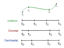
Let ${\displaystyle \mathbf {P} _{i}=[x_{i}\quad y_{i}]^{T}}$ denote a point. For a curve segment ${\displaystyle \mathbf {C} }$ defined by points ${\displaystyle \mathbf {P} _{0},\mathbf {P} _{1},\mathbf {P} _{2},\mathbf {P} _{3}}$ and knot sequence ${\displaystyle t_{0},t_{1},t_{2},t_{3}}$, the centripetal Catmull–Rom spline can be produced by:

${\displaystyle \mathbf {C} ={\frac {t_{2}-t}{t_{2}-t_{1}}}\mathbf {B} _{1}+{\frac {t-t_{1}}{t_{2}-t_{1}}}\mathbf {B} _{2}}$

where

${\displaystyle \mathbf {B} _{1}={\frac {t_{2}-t}{t_{2}-t_{0}}}\mathbf {A} _{1}+{\frac {t-t_{0}}{t_{2}-t_{0}}}\mathbf {A} _{2}}$

${\displaystyle \mathbf {B} _{2}={\frac {t_{3}-t}{t_{3}-t_{1}}}\mathbf {A} _{2}+{\frac {t-t_{1}}{t_{3}-t_{1}}}\mathbf {A} _{3}}$

${\displaystyle \mathbf {A} _{1}={\frac {t_{1}-t}{t_{1}-t_{0}}}\mathbf {P} _{0}+{\frac {t-t_{0}}{t_{1}-t_{0}}}\mathbf {P} _{1}}$

${\displaystyle \mathbf {A} _{2}={\frac {t_{2}-t}{t_{2}-t_{1}}}\mathbf {P} _{1}+{\frac {t-t_{1}}{t_{2}-t_{1}}}\mathbf {P} _{2}}$

${\displaystyle \mathbf {A} _{3}={\frac {t_{3}-t}{t_{3}-t_{2}}}\mathbf {P} _{2}+{\frac {t-t_{2}}{t_{3}-t_{2}}}\mathbf {P} _{3}}$

and

${\displaystyle t_{i+1}=\left[{\sqrt {(x_{i+1}-x_{i})^{2}+(y_{i+1}-y_{i})^{2}}}\right]^{\alpha }+t_{i}}$

in which ${\displaystyle \alpha }$ ranges from 0 to 1 for knot parameterization, and ${\displaystyle i=0,1,2,3}$ with ${\displaystyle t_{0}=0}$. For centripetal Catmull–Rom spline, the value of ${\displaystyle \alpha }$ is ${\displaystyle 0.5}$. When ${\displaystyle \alpha =0}$, the resulting curve is the standard uniform Catmull–Rom spline; when ${\displaystyle \alpha =1}$, the result is a chordal Catmull–Rom spline.

Plugging ${\displaystyle t=t_{1}}$ into the spline equations ${\displaystyle \mathbf {A} _{1},\mathbf {A} _{2},\mathbf {A} _{3},\mathbf {B} _{1},\mathbf {B} _{2},}$ and ${\displaystyle \mathbf {C} }$ shows that the value of the spline curve at ${\displaystyle t_{1}}$ is ${\displaystyle \mathbf {C} =\mathbf {P} _{1}}$. Similarly, substituting ${\displaystyle t=t_{2}}$ into the spline equations shows that ${\displaystyle \mathbf {C} =\mathbf {P} _{2}}$ at ${\displaystyle t_{2}}$. This is true independent of the value of ${\displaystyle \alpha }$ since the equation for ${\displaystyle t_{i+1}}$ is not needed to calculate the value of ${\displaystyle \mathbf {C} }$ at points ${\displaystyle t_{1}}$ and ${\displaystyle t_{2}}$.

The extension to 3D points is simply achieved by considering ${\displaystyle \mathbf {P} _{i}=[x_{i}\quad y_{i}\quad z_{i}]^{T}}$a generic 3D point ${\displaystyle \mathbf {P} _{i}}$ and

${\displaystyle t_{i+1}=\left[{\sqrt {(x_{i+1}-x_{i})^{2}+(y_{i+1}-y_{i})^{2}+(z_{i+1}-z_{i})^{2}}}\right]^{\alpha }+t_{i}}$

Advantages

Centripetal Catmull–Rom spline has several desirable mathematical properties compared to the original and the other types of Catmull-Rom formulation.^[3] First, it will not form loop or self-intersection within a curve segment. Second, cusp will never occur within a curve segment. Third, it follows the control points more tightly.^[4][vague]

Other uses

In computer vision, centripetal Catmull-Rom spline has been used to formulate an active model for segmentation. The method is termed active spline model.^[5] The model is devised on the basis of active shape model, but uses centripetal Catmull-Rom spline to join two successive points (active shape model uses simple straight line), so that the total number of points necessary to depict a shape is less. The use of centripetal Catmull-Rom spline makes the training of a shape model much simpler, and it enables a better way to edit a contour after segmentation.

Code example in Python

The following is an implementation of the Catmull–Rom spline in Python that produces the plot shown beneath.

import numpy
import matplotlib.pyplot as plt


QUADRUPLE_SIZE: int = 4


def num_segments(point_chain: tuple) -> int:
    # There is 1 segment per 4 points, so we must subtract 3 from the number of points  
    return len(point_chain) - (QUADRUPLE_SIZE - 1)


def flatten(list_of_lists) -> list:
    # E.g. mapping [[1, 2], [3], [4, 5]] to  [1, 2, 3, 4, 5] 
    return [elem for lst in list_of_lists for elem in lst]


def catmull_rom_spline(
    P0: tuple,
    P1: tuple,
    P2: tuple,
    P3: tuple,
    num_points: int,
    alpha: float = 0.5,
):
    """
    Compute the points in the spline segment
    :param P0, P1, P2, and P3: The (x,y) point pairs that define the Catmull-Rom spline
    :param num_points: The number of points to include in the resulting curve segment
    :param alpha: 0.5 for the centripetal spline, 0.0 for the uniform spline, 1.0 for the chordal spline.
    :return: The points
    """

    # Calculate t0 to t4. Then only calculate points between P1 and P2.
    # Reshape linspace so that we can multiply by the points P0 to P3
    # and get a point for each value of t.
    def tj(ti: float, pi: tuple, pj: tuple) -> float:
        xi, yi = pi
        xj, yj = pj
        dx, dy = xj - xi, yj - yi
        l = (dx ** 2 + dy ** 2) ** 0.5
        return ti + l ** alpha

    t0: float = 0.0
    t1: float = tj(t0, P0, P1)
    t2: float = tj(t1, P1, P2)
    t3: float = tj(t2, P2, P3)
    t = numpy.linspace(t1, t2, num_points).reshape(num_points, 1)

    A1 = (t1 - t) / (t1 - t0) * P0 + (t - t0) / (t1 - t0) * P1
    A2 = (t2 - t) / (t2 - t1) * P1 + (t - t1) / (t2 - t1) * P2
    A3 = (t3 - t) / (t3 - t2) * P2 + (t - t2) / (t3 - t2) * P3
    B1 = (t2 - t) / (t2 - t0) * A1 + (t - t0) / (t2 - t0) * A2
    B2 = (t3 - t) / (t3 - t1) * A2 + (t - t1) / (t3 - t1) * A3
    points = (t2 - t) / (t2 - t1) * B1 + (t - t1) / (t2 - t1) * B2
    return points


def catmull_rom_chain(points: tuple, num_points: int) -> list:
    """
    Calculate Catmull-Rom for a sequence of initial points and return the combined curve.
    :param points: Base points from which the quadruples for the algorithm are taken
    :param num_points: The number of points to include in each curve segment
    :return: The chain of all points (points of all segments)
    """
    point_quadruples = (  # Prepare function inputs
        (points[idx_segment_start + d] for d in range(QUADRUPLE_SIZE))
        for idx_segment_start in range(num_segments(points))
    )
    all_splines = (catmull_rom_spline(*pq, num_points) for pq in point_quadruples)
    return flatten(all_splines)


if __name__ == "__main__":
    POINTS: tuple = ((0, 1.5), (2, 2), (3, 1), (4, 0.5), (5, 1), (6, 2), (7, 3))  # Red points
    NUM_POINTS: int = 100  # Density of blue chain points between two red points

    chain_points: list = catmull_rom_chain(POINTS, NUM_POINTS)
    assert len(chain_points) == num_segments(POINTS) * NUM_POINTS  # 400 blue points for this example

    plt.plot(*zip(*chain_points), c="blue")
    plt.plot(*zip(*POINTS), c="red", linestyle="none", marker="o")
    plt.show()

Code example in Unity C#

using UnityEngine;

// a single catmull-rom curve
public struct CatmullRomCurve
{
	public Vector2 p0, p1, p2, p3;
	public float alpha;

	public CatmullRomCurve(Vector2 p0, Vector2 p1, Vector2 p2, Vector2 p3, float alpha)
   {
		(this.p0, this.p1, this.p2, this.p3) = (p0, p1, p2, p3);
		this.alpha = alpha;
	}

	// Evaluates a point at the given t-value from 0 to 1
	public Vector2 GetPoint(float t)
    {
		// calculate knots
		const float k0 = 0;
		float k1 = GetKnotInterval(p0, p1);
		float k2 = GetKnotInterval(p1, p2) + k1;
		float k3 = GetKnotInterval(p2, p3) + k2;

		// evaluate the point
		float u = Mathf.LerpUnclamped(k1, k2, t);
		Vector2 A1 = Remap(k0, k1, p0, p1, u);
		Vector2 A2 = Remap(k1, k2, p1, p2, u);
		Vector2 A3 = Remap(k2, k3, p2, p3, u);
		Vector2 B1 = Remap(k0, k2, A1, A2, u);
		Vector2 B2 = Remap(k1, k3, A2, A3, u);
		return Remap(k1, k2, B1, B2, u);
	}

	static Vector2 Remap(float a, float b, Vector2 c, Vector2 d, float u)
    {
		return Vector2.LerpUnclamped(c, d, (u - a) / (b - a));
	}

	float GetKnotInterval(Vector2 a, Vector2 b)
    {
		return Mathf.Pow(Vector2.SqrMagnitude(a - b), 0.5f * alpha);
	}
}

using UnityEngine;

// Draws a catmull-rom spline in the scene view,
// along the child objects of the transform of this component
public class CatmullRomSpline : MonoBehaviour
{
	[Range(0, 1)]
    public float alpha = 0.5f;
	int PointCount => transform.childCount;
	int SegmentCount => PointCount - 3;
	Vector2 GetPoint(int i) => transform.GetChild(i).position;

	CatmullRomCurve GetCurve(int i)
    {
		return new CatmullRomCurve(GetPoint(i), GetPoint(i+1), GetPoint(i+2), GetPoint(i+3), alpha);
	}

	void OnDrawGizmos()
    {
		for (int i = 0; i < SegmentCount; i++)
			DrawCurveSegment(GetCurve(i));
	}

	void DrawCurveSegment(CatmullRomCurve curve)
    {
		const int detail = 32;
		Vector2 prev = curve.p1;

		for (int i = 1; i < detail; i++)
        {
			float t = i / (detail - 1f);
			Vector2 pt = curve.GetPoint(t);
			Gizmos.DrawLine(prev, pt);
			prev = pt;
		}
	}
}

Code example in Unreal C++

float GetT( float t, float alpha, const FVector& p0, const FVector& p1 )
{
    auto d  = p1 - p0;
    float a = d | d; // Dot product
    float b = FMath::Pow( a, alpha*.5f );
    return (b + t);
}

FVector CatmullRom( const FVector& p0, const FVector& p1, const FVector& p2, const FVector& p3, float t /* between 0 and 1 */, float alpha=.5f /* between 0 and 1 */ )
{
    float t0 = 0.0f;
    float t1 = GetT( t0, alpha, p0, p1 );
    float t2 = GetT( t1, alpha, p1, p2 );
    float t3 = GetT( t2, alpha, p2, p3 );
    t = FMath::Lerp( t1, t2, t );
    FVector A1 = ( t1-t )/( t1-t0 )*p0 + ( t-t0 )/( t1-t0 )*p1;
    FVector A2 = ( t2-t )/( t2-t1 )*p1 + ( t-t1 )/( t2-t1 )*p2;
    FVector A3 = ( t3-t )/( t3-t2 )*p2 + ( t-t2 )/( t3-t2 )*p3;
    FVector B1 = ( t2-t )/( t2-t0 )*A1 + ( t-t0 )/( t2-t0 )*A2;
    FVector B2 = ( t3-t )/( t3-t1 )*A2 + ( t-t1 )/( t3-t1 )*A3;
    FVector C  = ( t2-t )/( t2-t1 )*B1 + ( t-t1 )/( t2-t1 )*B2;
    return C;
}

See also

• Cubic Hermite splines

References

External links

• Catmull-Rom curve with no cusps and no self-intersections – implementation in Java
• Catmull-Rom curve with no cusps and no self-intersections – simplified implementation in C++
• Catmull-Rom splines – interactive generation via Python, in a Jupyter notebook
• Smooth Paths Using Catmull-Rom Splines – another versatile implementation in C++ including centripetal CR splines

This page was last edited on 1 October 2023, at 13:41

References

- ^ Catmull, Edwin; Rom, Raphael (1974). "A class of local interpolating splines". In Barnhill, Robert E.; Riesenfeld, Richard F. (eds.). Computer Aided Geometric Design. pp. 317–326. doi:10.1016/B978-0-12-079050-0.50020-5. ISBN 978-0-12-079050-0.
- ^ Barry, Phillip J.; Goldman, Ronald N. (August 1988). A recursive evaluation algorithm for a class of Catmull–Rom splines. Proceedings of the 15st Annual Conference on Computer Graphics and Interactive Techniques, SIGGRAPH 1988. Vol. 22. Association for Computing Machinery. pp. 199–204. doi:10.1145/378456.378511.
- ^ Yuksel, Cem; Schaefer, Scott; Keyser, John (July 2011). "Parameterization and applications of Catmull-Rom curves". Computer-Aided Design. 43 (7): 747–755. CiteSeerX 10.1.1.359.9148. doi:10.1016/j.cad.2010.08.008.
- ^ Yuksel; Schaefer; Keyser, Cem; Scott; John. "On the Parameterization of Catmull-Rom Curves" (PDF).
{{cite web}}: CS1 maint: multiple names: authors list (link) - ^ Jen Hong, Tan; Acharya, U. Rajendra (2014). "Active spline model: A shape based model-interactive segmentation" (PDF). Digital Signal Processing. 35: 64–74. arXiv:1402.6387. doi:10.1016/j.dsp.2014.09.002. S2CID 6953844.