
In mathematics, particularly in dynamical systems, a bifurcation diagram shows the values visited or approached asymptotically (fixed points, periodic orbits, or chaotic attractors) of a system as a function of a bifurcation parameter in the system.[citation needed] It is usual to represent stable values with a solid line and unstable values with a dotted line, although often the unstable points are omitted. Bifurcation diagrams enable the visualization of bifurcation theory. In the context of discrete-time dynamical systems, the diagram is also called orbit diagram.


YouTube Encyclopedic
-
1/3Views:50 6251 9324 003
-
ODE | Bifurcation diagrams
-
Bifurcation Diagrams (Jeff's Office Hours)
-
Examples of phase diagrams and bifurcation diagrams
Transcription
I'll introduce now the idea of a 'bifurcation diagram'. Bifurcation diagrams are way study differential equations which may depend on some extra parameter. Now you've seen such a thing already. When I first introduced the Logistic equation I also discussed the addition of a harvesting term: this '-h'. So this differential equation would describe a population, 'x' governed by this Logistic model. But then I have a '-h' and that represents some constant rate of harvesting applied to the population, 'x'. Now the way to study such a thing, and how it depends on the parameter, 'h' is essentially to draw a lot of phase-lines. And we draw them for various values of the parameter, 'h'. So let's look first at the phase-line for 'h = 0'. So it looks like this: and the equilibria are at x = 0 and x = 10. And how I find those? Well, the equilibria are where dx/dt = 0. So I take this right-hand side and I set it equal to '0'. And I remember that I've set h = 0 in order to draw this phase-line, So I have (1/10)*x*(10 - x) - 0 = 0 and that means x = 10 and x = 0. So those are the two equilibria. And then I can test of the sign of 'dx/dt' above x = 10 by plugging it in this right-hand side again with 'h = 0'. And I find it's negative, so the solution goes down. In-between x = 0 and 10, it's positive, so the solution goes up, And below x = 0 dx/dt is negative, so the solution goes down. How about the phase-line for 'h = 1'? I did 'h = 0' right here, so I'll move over one unit and do 'h = 1' right here. Now it looks roughly the same, except the two equilibria have moved in a little bit more And how I know that? Well I set h = 1 in this equation and I get (1/10)*x*(10 - x) - 1 = 0, and solve for the two x values - which are the equilibria. And those guys are at: x = 5 + 10^(1/2) and x = 5 - 10^(1/2). So you see that they've moved in a little closer just inched in toward.. '5' Okay, how about 'h = 2'? At h = 2 something kind of special happens: I only have one equilibrium value. And above and below that equilibrium dx/dt will be negative. I no longer have an area where dx/dt is positive, like on the two previous phase-lines. And, where do I get all this information? Well, I set 'h = 2' in the right-hand side of this equation, and I get (1/10)*x*(10 - x) - 2 = 0. There's only one route to that equation: that's 'x = 5' and I can test that this quantity is negative for x > 5, and negative for x < 5. I can keep drawing more phase-lines, for instance 'h = 3' I'll find there are no equilibria and, everywhere, dx/dt is negative. And, again, I find that by simply plugging in 'h = 3' into the right-hand side of the equation, setting it equal to '0', and finding there are no real-roots 'x' and hence no equilibria. In fact that quantity on the right-hand side is always negative hence the arrow is pointing down everywhere. Okay I've taken away all the calculations What we're left with is the beginning of a bifurcation diagram. I've drawn phase-lines for various values of 'h' And we can see in those phase-lines the bifurcation - or the 'splitting' of equilibria. For instance, at 'h= 3', we have no equilibrium values. At 'h = 2', one equilibrium appears. Then, at 'h = 1' we have two equilibria. At 'h = 0' I still have two [equilbria] Now, you can imagine drawing in other phase-lines, in between these: say at 'h = 0.5' or 'h = 1.5' (etc.) And we'd (sort of) get a 'smooth' picture of the way that these equilibrium values split and begin to move apart. So I can draw that smooth line in (it's a parabola in fact.) And how do I know it's a parabola? Well, it's exactly described by this equation: (1/10)*x*(10 - x) - h = 0. And that is a parabola in the x,h plane So if I draw in these axes, here, make this the 'h-axis' and these are the various values of the 'h' that I've chosen, h = 0... h = 1... h = 2 (etc) and this is the x-axis represented by the vertical position on the phase-line, then that's the parabola: it's a sideways-parabola given by this equation. So that pretty much completes our picture. We now have a bifurcation diagram, which is the bifurcation diagram for the example equation that I gave, and that is the Logistic equation with some harvesting parameter, 'h'. And we can use that bifurcation diagram to study how this Logistic model depends on the harvesting, 'h'. And if you remember, that was our original goal: to study how an ODE depends on a parameter. And in fact we can answer some questions about 'harvesting-rates'. Now let's suppose (just to make things a little more real) that 'x' represents a population of fish let's say in some lake. So that means, without any harvesting, that the population of fish is governed by a Logistic model, given here. Now, 'h' would represent some fishing-rate: some rate at which I catch fish and remove them from the lake. Now my question for you would be: what is the maximum sustainable fishing-rate? At what rate do I know that I can fish without killing off the fish population entirely?
Logistic map
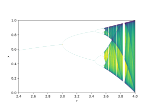
An example is the bifurcation diagram of the logistic map:

The bifurcation parameter r is shown on the horizontal axis of the plot and the vertical axis shows the set of values of the logistic function visited asymptotically from almost all initial conditions.
The bifurcation diagram shows the forking of the periods of stable orbits from 1 to 2 to 4 to 8 etc. Each of these bifurcation points is a period-doubling bifurcation. The ratio of the lengths of successive intervals between values of r for which bifurcation occurs converges to the first Feigenbaum constant.
The diagram also shows period doublings from 3 to 6 to 12 etc., from 5 to 10 to 20 etc., and so forth.
Symmetry breaking in bifurcation sets

In a dynamical system such as


Applications
Consider a system of differential equations that describes some physical quantity, that for concreteness could represent one of three examples: 1. the position and velocity of an undamped and frictionless pendulum, 2. a neuron's membrane potential over time, and 3. the average concentration of a virus in a patient's bloodstream. The differential equations for these examples include *parameters* that may affect the output of the equations. Changing the pendulum's mass and length will affect its oscillation frequency, changing the magnitude of injected current into a neuron may transition the membrane potential from resting to spiking, and the long-term viral load in the bloodstream may decrease with carefully timed treatments.
In general, researchers may seek to quantify how the long-term (asymptotic) behavior of a system of differential equations changes if a parameter is changed. In the dynamical systems branch of mathematics, a bifurcation diagram quantifies these changes by showing how fixed points, periodic orbits, or chaotic attractors of a system change as a function of bifurcation parameter. Bifurcation diagrams are used to visualize these changes.
See also
Further reading
- Glendinning, Paul (1994). Stability, Instability and Chaos. Cambridge University Press. ISBN 0-521-41553-5.
- May, Robert M. (1976). "Simple mathematical models with very complicated dynamics". Nature. 261 (5560): 459–467. Bibcode:1976Natur.261..459M. doi:10.1038/261459a0. hdl:10338.dmlcz/104555. PMID 934280. S2CID 2243371.
- Strogatz, Steven (2000). Non-linear Dynamics and Chaos: With applications to Physics, Biology, Chemistry and Engineering. Perseus Books. ISBN 0-7382-0453-6.
External links
- The Logistic Map and Chaos by Elmer G. Wiens, egwald.ca
- Wikiversity: Discrete-time dynamical system orbit diagram
This chaos theory-related article is a stub. You can help Wikipedia by expanding it. |