
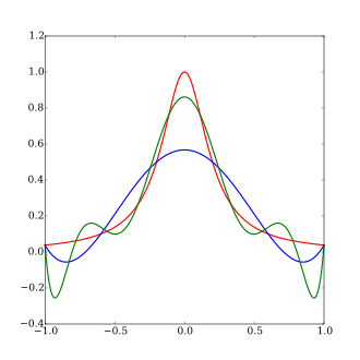
The function

A fifth order polynomial interpolation (exact replication of the red curve at 6 points)
A ninth order polynomial interpolation (exact replication of the red curve at 10 points)
In the mathematical field of numerical analysis, Runge's phenomenon (German: [ˈʁʊŋə]) is a problem of oscillation at the edges of an interval that occurs when using polynomial interpolation with polynomials of high degree over a set of equispaced interpolation points. It was discovered by Carl David Tolmé Runge (1901) when exploring the behavior of errors when using polynomial interpolation to approximate certain functions.[1] The discovery shows that going to higher degrees does not always improve accuracy. The phenomenon is similar to the Gibbs phenomenon in Fourier series approximations.
YouTube Encyclopedic
-
1/5Views:2 6091 738458 68915 9328 667
-
Higher Order Interpolation is a Bad Idea
-
Spline interpolation in ArcGIS
-
Euler's method | First order differential equations | Khan Academy
-
R11. Double Pendulum System
-
Lecture - 7 The Chua's Circuit
Transcription
. . . . In this segment we're going to talk about why higher order interpolation is a bad idea. This was an experiment which was conducted by Runge, who was a German mathematician, and had a lot of contributions to numerical methods.|In 1901, what he wanted to show was that higher order interpolation is a bad idea.|So he took a simple function, which you are seeing here, 1 divided by 1 plus 25 x squared, and what we did was he said, hey, let me go ahead and take, let's suppose, six data points which are equidistantly spaced. So you have six data points which are equidistantly spaced on this function of 1 divided by 1 plus 25 x squared, from -1 to +1, and this blue line, which is shown there, is simply the function itself, so that's the original function.|So the six data points are given in the table here, right from the function itself, and what we wanted to do was to say that, hey, let me take these six data points, and let a fifth-order polynomial pass through those six data points. Because you have six data points, you can take a fifth-order polynomial and make it go through those six data points.|And this is what he obtained, so here what you are finding out that you have these six data points which you have, and the blue line which you are seeing here is the original function.|So the blue line is the original function, and the red line which you're seeing here is basically the fifth-order polynomial going through those six data points.|And you're already finding out there's a vast difference between what you get as the interpolated value at, let's suppose at x equal to 0, and what you have as the value at x equal to 1.|So fifth-order polynomial turns out to be not a good approximation for the original function, 1 divided by 1 plus 25 x squared.|So people thought that maybe . . . Runge thought that maybe it's because he's not taking enough data points from -1 to +1, maybe he should take more data points, and most probably what's going to happen is that the interpolant is going to be closer to the original function.|So this is what he did was that he said let me go ahead and take twenty data points now, which are equidistantly spaced from -1 to +1. So if you're taking twenty data points, as shown in the graph there, now what you want to do is you want to take those twenty data points, and let a nineteenth-order polynomial pass through those twenty data points.|So let's see what happens now.|And you can see that it's worse now. So you're finding out that your original function is the blue line, the interpolant, the nineteenth-order polynomial which you are seeing here is the red line, and you're already finding out the red line is giving you values which are astronomical, as opposed to what they originally are at these endpoints there.|So you're finding out that higher order interpolation's a bad idea.|In fact, if you take more and more data points equidistantly spaced from -1 to +1, what's going to happen is that you're going to get even more error in the interpolant between the function value and the interpolant value itself, especially at the endpoints.|What you are finding out is that as you take more data points, yes, between about maybe -0.7 and +0.7, you're finding out that the original function and the interpolant itself are matching, but it's at the endpoints where you're having the problem where you get the largest difference between the interpolant and the Runge's function itself.|So what is the antidote to this problem?|It is something called spline interpolation.|Spline interpolation is explained in a separate segment, and what we are finding out here is that if we do spline interpolation for the same twenty data points which we had in the previous graph, that the spline interpolant, which is the green curve which you are seeing here, you cannot see the blue line itself.|The blue line is the original function, and the reason why you're not able to see the blue line is because the original function and the spline are almost on top of each other.|So you're finding out that this cubic spline interpolation . . . interpolant which has been drawn through the twenty data points which were chosen for the interpolant, do a better job of interpolating the function, as opposed to . . . as opposed to the nineteenth-order polynomial. So this also shows you that spline interpolation is the answer to higher order interpolation, which might be a bad idea.|Now, there's a Wolfram demonstration which has been . . . which is being shown here with permission from Wolfram Research, who are the makers of Mathematica.|So what they have done is that they have made these demonstrations using Mathematica, something called Mathematica player, where they basically give you an interactive simulation of the Runge's phenomenon, which I just showed it to you through some graphs.|So let's go ahead and go through those and see that how, as we keep on increasing the polynomial interpolant, do we get . . . do we get a better . . . better approximation. So here we have . . . we are choosing equally spaced data points, and now this is a fifth-order polynomial which I . . . fourth-order polynomial going through the function itself.|So you have the function, 1 divided by 1 plus 25 x squared, you are choosing four data points . . . five data points, and you're passing a fifth-order . . . fourth-order polynomial through the data points.|At the bottom, there's a graph which shows you what the . . . what the error in the interpolant is, and in this case, the maximum error which you're getting is about 0.5 or so.|Now, if I increase the . . . increase the . . . increase the number of data points which I'm choosing.|So let's suppose if I'm choosing 25 data points now, which means that a 24th-order polynomial is going through those data points, and already you're finding out that at the endpoints, you are getting a large difference between the interpolant and the function itself, and the error in the interpolant is about 250 or so.|So as you keep on increasing the order of the polynomial, you find out that you're getting more and more error, the difference between the maximum error which you're getting in the interpolant is becoming more and more.|In fact, I can increase it . . . increase it all the way up to 50, because the simulation allows you to have 50 data points, so it's a 49th-order polynomial.|So in the 49th-order polynomial, the amount of error which you're getting in the interpolant is about 700000.|So you can very well see that the large difference which you're getting between the interpolant values and the function itself is about 700000, and it increases as you keep on increasing . . . keeping on increasing more and more data points.|Now, in this Wolfram demonstration, there's a good thing which has been shown there is that you have an option of choosing Chebyshev points.|So if I move this to Chebyshev points, you are finding out that you are getting a better interpolant than what you had previously.|So here, now, the error, which was 700000, the maximum error which you are getting is 0.0001. So what is the difference between the Chebyshev points and the equally spaced points which are used in this demonstration? It is that the Chebyshev points are skewed more towards the endpoints.|You have more . . . more points chosen for interpolation near the ends, as opposed to equally spaced, as we had previously, and this seems to answer the question that, hey, if we want to reduce the amount of error between the original function and the . . . and the . . . original function and the interpolant, that we need to choose Chebyshev points to be able to do that. Now, one of the things which you might be asking is that, hey, is there a similar scheme which I can use for any continuous function?|No, Faber, a great mathematician, he showed in a theorem that there is no specific way, no general way which you can come up with how to choose data points to approximate a curve without getting into too much error between the interpolant and the function itself. But in this particular case, for this particular function, 1 divided by 1 plus 25 x squared, the Chebyshev points do work the best in terms of reducing the amount of error between the interpolant and the function itself.|And that's the end of this segment. . . .
Introduction
The Weierstrass approximation theorem states that for every continuous function f(x) defined on an interval [a,b], there exists a set of polynomial functions Pn(x) for n=0, 1, 2, ..., each of degree at most n, that approximates f(x) with uniform convergence over [a,b] as n tends to infinity, that is,

Consider the case where one desires to interpolate through n+1 equispaced points of a function f(x) using the n-degree polynomial Pn(x) that passes through those points. Naturally, one might expect from Weierstrass' theorem that using more points would lead to a more accurate reconstruction of f(x). However, this particular set of polynomial functions Pn(x) is not guaranteed to have the property of uniform convergence; the theorem only states that a set of polynomial functions exists, without providing a general method of finding one.
The Pn(x) produced in this manner may in fact diverge away from f(x) as n increases; this typically occurs in an oscillating pattern that magnifies near the ends of the interpolation points. The discovery of this phenomenon is attributed to Runge.[2]
Problem
Consider the Runge function

(a scaled version of the Witch of Agnesi). Runge found that if this function is interpolated at equidistant points xi between −1 and 1 such that:

with a polynomial Pn(x) of degree ≤ n, the resulting interpolation oscillates toward the end of the interval, i.e. close to −1 and 1. It can even be proven that the interpolation error increases (without bound) when the degree of the polynomial is increased:

This shows that high-degree polynomial interpolation at equidistant points can be troublesome.
Reason
Runge's phenomenon is the consequence of two properties of this problem.
- The magnitude of the n-th order derivatives of this particular function grows quickly when n increases.
- The equidistance between points leads to a Lebesgue constant that increases quickly when n increases.
The phenomenon is graphically obvious because both properties combine to increase the magnitude of the oscillations.
The error between the generating function and the interpolating polynomial of order n is given by

for some in (−1, 1). Thus,

- .

Denote by the nodal function


and let be the maximum of the magnitude of the function:


- .

It is elementary to prove that with equidistant nodes

where is the step size.

Moreover, assume that the (n+1)-th derivative of is bounded, i.e.

- .

Therefore,
- .

But the magnitude of the (n+1)-th derivative of Runge's function increases when n increases. The consequence is that the resulting upper bound tends to infinity when n tends to infinity.
Although often used to explain the Runge phenomenon, the fact that the upper bound of the error goes to infinity does not necessarily imply, of course, that the error itself also diverges with n.
Mitigations
Change of interpolation points
The oscillation can be minimized by using nodes that are distributed more densely towards the edges of the interval, specifically, with asymptotic density (on the interval [−1, 1]) given by the formula[3] . A standard example of such a set of nodes is Chebyshev nodes, for which the maximum error in approximating the Runge function is guaranteed to diminish with increasing polynomial order.

S-Runge algorithm without resampling
When equidistant samples must be used because resampling on well-behaved sets of nodes is not feasible, the S-Runge algorithm can be considered.[4] In this approach, the original set of nodes is mapped on the set of Chebyshev nodes, providing a stable polynomial reconstruction. The peculiarity of this method is that there is no need of resampling at the mapped nodes, which are also called fake nodes. A Python implementation of this procedure can be found here.
Use of piecewise polynomials
The problem can be avoided by using spline curves which are piecewise polynomials. When trying to decrease the interpolation error one can increase the number of polynomial pieces which are used to construct the spline instead of increasing the degree of the polynomials used.
Constrained minimization
One can also fit a polynomial of higher degree (for instance, with points use a polynomial of order instead of ), and fit an interpolating polynomial whose first (or second) derivative has minimal norm.


A similar approach is to minimize a constrained version of the distance between the polynomial's -th derivative and the mean value of its -th derivative. Explicitly, to minimize


where and , with respect to the polynomial coefficients and the Lagrange multipliers, . When , the constraint equations generated by the Lagrange multipliers reduce to the minimum polynomial that passes through all points. At the opposite end, will approach a form very similar to a piecewise polynomials approximation. When , in particular, approaches the linear piecewise polynomials, i.e. connecting the interpolation points with straight lines.


The role played by in the process of minimizing is to control the importance of the size of the fluctuations away from the mean value. The larger is, the more large fluctuations are penalized compared to small ones. The greatest advantage of the Euclidean norm, , is that it allows for analytic solutions and it guarantees that will only have a single minimum. When there can be multiple minima in , making it difficult to ensure that a particular minimum found will be the global minimum instead of a local one.


Least squares fitting
Another method is fitting a polynomial of lower degree using the method of least squares. Generally, when using equidistant points, if then least squares approximation is well-conditioned.[5]

Bernstein polynomial
Using Bernstein polynomials, one can uniformly approximate every continuous function in a closed interval, although this method is rather computationally expensive.[citation needed]
External fake constraints interpolation
This method proposes to optimally stack a dense distribution of constraints of the type P″(x) = 0 on nodes positioned externally near the endpoints of each side of the interpolation interval, where P"(x) is the second derivative of the interpolation polynomial. Those constraints are called External Fake Constraints as they do not belong to the interpolation interval and they do not match the behaviour of the Runge function. The method has demonstrated that it has a better interpolation performance than Piecewise polynomials (splines) to mitigate the Runge phenomenon.[6]
Related statements from the approximation theory
For every predefined table of interpolation nodes there is a continuous function for which the sequence of interpolation polynomials on those nodes diverges.[7] For every continuous function there is a table of nodes on which the interpolation process converges. [citation needed] Chebyshev interpolation (i.e., on Chebyshev nodes) converges uniformly for every absolutely continuous function.
See also
- Chebyshev nodes
- Compare with the Gibbs phenomenon for sinusoidal basis functions
- Occam's razor argues for simpler models
- Overfitting can be caused by excessive model complexity
- Schwarz lantern, another example of failure of convergence
- Stone–Weierstrass theorem
- Taylor series
- Wilkinson's polynomial
References
- ^ Runge, Carl (1901), "Über empirische Funktionen und die Interpolation zwischen äquidistanten Ordinaten", Zeitschrift für Mathematik und Physik, 46: 224–243. available at www.archive.org
- ^ Epperson, James (1987). "On the Runge example". Amer. Math. Monthly. 94: 329–341. doi:10.2307/2323093.
- ^ Berrut, Jean-Paul; Trefethen, Lloyd N. (2004), "Barycentric Lagrange interpolation", SIAM Review, 46 (3): 501–517, CiteSeerX 10.1.1.15.5097, doi:10.1137/S0036144502417715, ISSN 1095-7200
- ^ De Marchi, Stefano; Marchetti, Francesco; Perracchione, Emma; Poggiali, Davide (2020), "Polynomial interpolation via mapped bases without resampling", J. Comput. Appl. Math., 364, doi:10.1016/j.cam.2019.112347, ISSN 0377-0427
- ^ Dahlquist, Germund; Björk, Åke (1974), "4.3.4. Equidistant Interpolation and the Runge Phenomenon", Numerical Methods, pp. 101–103, ISBN 0-13-627315-7
- ^ Belanger, Nicolas (2017), External Fake Constraints Interpolation: the end of Runge phenomenon with high degree polynomials relying on equispaced nodes – Application to aerial robotics motion planning (PDF), Proceedings of the 5th Institute of Mathematics and its Applications Conference on Mathematics in Defence
- ^ Cheney, Ward; Light, Will (2000), A Course in Approximation Theory, Brooks/Cole, p. 19, ISBN 0-534-36224-9