
| Part of a series on |
| Regression analysis |
|---|
| Models |
| Estimation |
| Background |

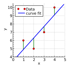
Least-squares spectral analysis (LSSA) is a method of estimating a frequency spectrum based on a least-squares fit of sinusoids to data samples, similar to Fourier analysis.[1][2] Fourier analysis, the most used spectral method in science, generally boosts long-periodic noise in the long and gapped records; LSSA mitigates such problems.[3] Unlike in Fourier analysis, data need not be equally spaced to use LSSA.
Developed in 1969[4] and 1971,[5] LSSA is also known as the Vaníček method and the Gauss-Vaniček method after Petr Vaníček,[6][7] and as the Lomb method[3] or the Lomb–Scargle periodogram,[2][8] based on the simplifications first by Nicholas R. Lomb[9] and then by Jeffrey D. Scargle.[10]
YouTube Encyclopedic
-
1/5Views:467 87913 0741 0416 035 38112 542
-
Least squares approximation | Linear Algebra | Khan Academy
-
11: Spectral Analysis Part 1 - Intro to Neural Computation
-
Spectral Numerical Method
-
The Real Meaning of E=mc²
-
Lec 4 | MIT 18.085 Computational Science and Engineering I
Transcription
Let's say I have some matrix A. Let's say it's an n-by-k matrix, and I have the equation Ax is equal to b. So in this case, x would have to be a member of Rk, because we have k columns here, and b is a member of Rn. Now, let's say that it just so happens that there is no solution to Ax is equal to b. What does that mean? Let's just expand out A. I think you already know what that means. If I write a like this, a1, a2, if I just write it as its columns vectors right there, all the way through ak, and then I multiply it times x1, x2, all the way through xk, this is the same thing as that equation there. I just kind of wrote out the two matrices. Now, this is the same thing as x1 times a1 plus x2 times a2, all the way to plus xk times ak is equal to the vector b. Now, if this has no solution, then that means that there's no set of weights here on the column vectors of a, where we can get to b. Or another way to say it is, no linear combinations of the column vectors of a will be equal to b. Or an even further way of saying it is that b is not in the column space of a. No linear combination of these guys can equal to that. So let's see if we can visualize it a bit. So let me draw the column space of a. So maybe the column space of a looks something like this right here. I'll just assume it's a plane in Rn. It doesn't have to be a plane. Things can be very general, but let's say that this is the column space. This is the column space of a. Now, if that's the column space and b is not in the column space, maybe we can draw b like this. Maybe b, let's say this is the origin right there, and b just pops out right there. So this is the 0 vector. This is my vector b, clearly not in my column spaces, clearly not in this plane. Now, up until now, we would get an equation like that. We would make an augmented matrix, put in reduced row echelon form, and get a line that said 0 equals 1, and we'd say, no solution, nothing we can do here. But what if we can do better? You know, we clearly can't find a solution to this. But what if we can find a solution that gets us close to this? So what if I want to find some x, I'll call it x-star for now, where-- so I want to find some x-star, where A times x-star is-- and this is a vector-- as close as possible-- let me write this-- as close to b as possible. Or another way to view it, when I say close, I'm talking about length, so I want to minimize the length of-- let me write this down. I want to minimize the length of b minus A times x-star. Now, some of you all might already know where this is going. But when you take the difference between 2 and then take its length, what does that look like? Let me just call Ax. Ax is going to be a member of my column space. Let me just call that v. Ax is equal to v. You multiply any vector in Rk times your matrix A, you're going to get a member of your column space. So any Ax is going to be in your column space. And maybe that is the vector v is equal to A times x-star. And we want this vector to get as close as possible to this as long as it stays-- I mean, it has to be in my column space. But we want the distance between this vector and this vector to be minimized. Now, I just want to show you where the terminology for this will come from. I haven't given it its proper title yet. If you were to take this vector-- let just call this vector v for simplicity-- that this is equivalent to the length of the vector. You take the difference between each of the elements. So b1 minus v1, b2 minus v2, all the way to bn minus vn. And if you take the length of this vector, this is the same thing as this. This is going to be equal to the square root. Let me take the length squared, actually. The length squared of this is just going to be b1 minus v1 squared plus b2 minus v2 squared plus all the way to bn minus vn squared. And I want to minimize this. So I want to make this value the least value that it can be possible, or I want to get the least squares estimate here. And that's why, this last minute or two when I was just explaining this, that was just to give you the motivation for why this right here is called the least squares estimate, or the least squares solution, or the least squares approximation for the equation Ax equals b. There is no solution to this, but maybe we can find some x-star, where if I multiply A times x-star, this is clearly going to be in my column space and I want to get this vector to be as close to b as possible. Now, we've already seen in several videos, what is the closest vector in any subspace to a vector that's not in my subspace? Well, the closest vector to it is the projection. The closest vector to b, that's in my subspace, is going to be the projection of b onto my column space. That is the closest vector there. So if I want to minimize this, I want to figure out my x-star, where Ax-star is equal to the projection of my vector b onto my subspace or onto the column space of A. Remember what we're doing here. We said Axb has no solution, but maybe we can find some x that gets us as close as possible. So I'm calling that my least squares solution or my least squares approximation. And this guy right here is clearly going to be in my column space, because you take some vector x times A, that's going to be a linear combination of these column vectors, so it's going to be in the column space. And I want this guy to be as close as possible to this guy. Well, the closest vector in my column space to that guy is the projection. So Ax needs to be equal to the projection of b on my column space. It needs to be equal to that. But this is still pretty hard to find. You saw how, you know, you took A times the inverse of A transpose A times A transpose. That's hard to find that transformation matrix. So let's see if we can find an easier way to figure out the least squares solution, or kind of our best solution. It's not THE solution. It's our BEST solution to this right here. That's why we call it the least squares solution or approximation. Let's just subtract b from both sides of this and we might get something interesting. So what happens if we take Ax minus the vector b on both sides of this equation? I'll do it up here on the right. On the left-hand side we get A times x-star. It's hard write the x and then the star because they're very similar. And we subtract b from it. We subtract our vector b. That's going to be equal to the projection of b onto our column space minus b. All I did is I subtracted b from both sides of this equation. Now, what is the projection of b minus our vector b? If we draw it right here, it's going to be this vector right-- let me do it in this orange color. It's going to be this right here. It's going to be that vector right there, right? If I take the projection of b, which is that, minus b, I'm going to get this vector. you we could say b plus this vector is equal to my projection of b onto my subspace. So this vector right here is orthogonal. It's actually part of the definition of a projection that this guy is going to be orthogonal to my subspace or to my column space. And so this guy is orthogonal to my column space. So I can write Ax-star minus b, it's orthogonal to my column space, or we could say it's a member of the orthogonal complement of my column space. The orthogonal complement is just the set of everything, all of the vectors that are orthogonal to everything in your subspace, in your column space right here. So this vector right here that's kind of pointing straight down onto my plane is clearly a member of the orthogonal complement of my column space. Now, this might look familiar to you already. What is the orthogonal complement of my column space? The orthogonal complement of my column space is equal to the null space of a transpose, or the left null space of A. We've done this in many, many videos. So we can say that A times my least squares estimate of the equation Ax is equal to b-- I wrote that. So x-star is my least squares solution to Ax is equal to b. So A times that minus b is a member of the null space of A transpose. Now, what does that mean? Well, that means that if I multiply A transpose times this guy right here, times Ax-star-- and let me, no I don't want to lose the vector signs there on the x. This is a vector. I don't want to forget that. Ax-star minus b. So if I multiply A transpose times this right there, that is the same thing is that, what am I going to get? Well, this is a member of the null space of A transpose, so this times A transpose has got to be equal to 0. It is a solution to A transpose times something is equal to the 0 vector. Now. Let's see if we can simplify this a little bit. We get A transpose A times x-star minus A transpose b is equal to 0, and then if we add this term to both sides of the equation, we are left with A transpose A times the least squares solution to Ax equal to b is equal to A transpose b. That's what we get. Now, why did we do all of this work? Remember what we started with. We said we're trying to find a solution to Ax is equal to b, but there was no solution. So we said, well, let's find at least an x-star that minimizes b, that minimizes the distance between b and Ax-star. And we call this the least squares solution. We call it the least squares solution because, when you actually take the length, or when you're minimizing the length, you're minimizing the squares of the differences right there. So it's the least squares solution. Now, to find this, we know that this has to be the closest vector in our subspace to b. And we know that the closest vector in our subspace to b is the projection of b onto our subspace, onto our column space of A. And so, we know that A-- let me switch colors. We know that A times our least squares solution should be equal to the projection of b onto the column space of A. If we can find some x in Rk that satisfies this, that is our least squares solution. But we've seen before that the projection b is easier said than done. You know, there's a lot of work to it. So maybe we can do it a simpler way. And this is our simpler way. If we're looking for this, alternately, we can just find a solution to this equation. So you give me an Ax equal to b, there is no solution. Well, what I'm going to do is I'm just going to multiply both sides of this equation times A transpose. If I multiply both sides of this equation by A transpose, I get A transpose times Ax is equal to A transpose-- and I want to do that in the same blue-- A-- no, that's not the same blue-- A transpose b. All I did is I multiplied both sides of this. Now, the solution to this equation will not be the same as the solution to this equation. This right here will always have a solution, and this right here is our least squares solution. So this right here is our least squares solution. And notice, this is some matrix, and then this right here is some vector. This right here is some vector. So long as we can find a solution here, we've given our best shot at finding a solution to Ax equal to b. We've minimized the error. We're going to get Ax-star, and the difference between Ax-star and b is going to be minimized. It's going to be our least squares solution. It's all a little bit abstract right now in this video, but hopefully, in the next video, we'll realize that it's actually a very, very useful concept.
Historical background
The close connections between Fourier analysis, the periodogram, and the least-squares fitting of sinusoids have been known for a long time.[11] However, most developments are restricted to complete data sets of equally spaced samples. In 1963, Freek J. M. Barning of Mathematisch Centrum, Amsterdam, handled unequally spaced data by similar techniques,[12] including both a periodogram analysis equivalent to what nowadays is called the Lomb method and least-squares fitting of selected frequencies of sinusoids determined from such periodograms — and connected by a procedure known today as the matching pursuit with post-back fitting[13] or the orthogonal matching pursuit.[14]
Petr Vaníček, a Canadian geophysicist and geodesist of the University of New Brunswick, proposed in 1969 also the matching-pursuit approach for equally and unequally spaced data, which he called "successive spectral analysis" and the result a "least-squares periodogram".[4] He generalized this method to account for any systematic components beyond a simple mean, such as a "predicted linear (quadratic, exponential, ...) secular trend of unknown magnitude", and applied it to a variety of samples, in 1971.[5]
Vaníček's strictly least-squares method was then simplified in 1976 by Nicholas R. Lomb of the University of Sydney, who pointed out its close connection to periodogram analysis.[9] Subsequently, the definition of a periodogram of unequally spaced data was modified and analyzed by Jeffrey D. Scargle of NASA Ames Research Center,[10] who showed that, with minor changes, it becomes identical to Lomb's least-squares formula for fitting individual sinusoid frequencies.
Scargle states that his paper "does not introduce a new detection technique, but instead studies the reliability and efficiency of detection with the most commonly used technique, the periodogram, in the case where the observation times are unevenly spaced," and further points out regarding least-squares fitting of sinusoids compared to periodogram analysis, that his paper "establishes, apparently for the first time, that (with the proposed modifications) these two methods are exactly equivalent."[10]
Press[3] summarizes the development this way:
A completely different method of spectral analysis for unevenly sampled data, one that mitigates these difficulties and has some other very desirable properties, was developed by Lomb, based in part on earlier work by Barning and Vanicek, and additionally elaborated by Scargle.
In 1989, Michael J. Korenberg of Queen's University in Kingston, Ontario, developed the "fast orthogonal search" method of more quickly finding a near-optimal decomposition of spectra or other problems,[15] similar to the technique that later became known as the orthogonal matching pursuit.
Development of LSSA and variants
The Vaníček method
In the Vaníček method, a discrete data set is approximated by a weighted sum of sinusoids of progressively determined frequencies using a standard linear regression or least-squares fit.[16] The frequencies are chosen using a method similar to Barning's, but going further in optimizing the choice of each successive new frequency by picking the frequency that minimizes the residual after least-squares fitting (equivalent to the fitting technique now known as matching pursuit with pre-backfitting[13]). The number of sinusoids must be less than or equal to the number of data samples (counting sines and cosines of the same frequency as separate sinusoids).
A data vector Φ is represented as a weighted sum of sinusoidal basis functions, tabulated in a matrix A by evaluating each function at the sample times, with weight vector x:
- ,

where the weights vector x is chosen to minimize the sum of squared errors in approximating Φ. The solution for x is closed-form, using standard linear regression:[17]

Here the matrix A can be based on any set of functions mutually independent (not necessarily orthogonal) when evaluated at the sample times; functions used for spectral analysis are typically sines and cosines evenly distributed over the frequency range of interest. If we choose too many frequencies in a too-narrow frequency range, the functions will be insufficiently independent, the matrix ill-conditioned, and the resulting spectrum meaningless.[17]
When the basis functions in A are orthogonal (that is, not correlated, meaning the columns have zero pair-wise dot products), the matrix ATA is diagonal; when the columns all have the same power (sum of squares of elements), then that matrix is an identity matrix times a constant, so the inversion is trivial. The latter is the case when the sample times are equally spaced and sinusoids chosen as sines and cosines equally spaced in pairs on the frequency interval 0 to a half cycle per sample (spaced by 1/N cycles per sample, omitting the sine phases at 0 and maximum frequency where they are identically zero). This case is known as the discrete Fourier transform, slightly rewritten in terms of measurements and coefficients.[17]
- — DFT case for N equally spaced samples and frequencies, within a scalar factor.

The Lomb method
Trying to lower the computational burden of the Vaníček method in 1976 [9] (no longer an issue), Lomb proposed using the above simplification in general, except for pair-wise correlations between sine and cosine bases of the same frequency, since the correlations between pairs of sinusoids are often small, at least when they are not tightly spaced. This formulation is essentially that of the traditional periodogram but adapted for use with unevenly spaced samples. The vector x is a reasonably good estimate of an underlying spectrum, but since we ignore any correlations, Ax is no longer a good approximation to the signal, and the method is no longer a least-squares method — yet in the literature continues to be referred to as such.
Rather than just taking dot products of the data with sine and cosine waveforms directly, Scargle modified the standard periodogram formula so to find a time delay first, such that this pair of sinusoids would be mutually orthogonal at sample times and also adjusted for the potentially unequal powers of these two basis functions, to obtain a better estimate of the power at a frequency.[3][10] This procedure made his modified periodogram method exactly equivalent to Lomb's method. Time delay by definition equals to


Then the periodogram at frequency is estimated as:

- ,
![{\displaystyle P_{x}(\omega )={\frac {1}{2}}\left({\frac {\left[\sum _{j}X_{j}\cos \omega (t_{j}-\tau )\right]^{2}}{\sum _{j}\cos ^{2}\omega (t_{j}-\tau )}}+{\frac {\left[\sum _{j}X_{j}\sin \omega (t_{j}-\tau )\right]^{2}}{\sum _{j}\sin ^{2}\omega (t_{j}-\tau )}}\right)}](https://wikimedia.org/api/rest_v1/media/math/render/svg/36fbcce2dc02ce0426d6b6b859ba15cbeba9abc6)
which, as Scargle reports, has the same statistical distribution as the periodogram in the evenly sampled case.[10]
At any individual frequency , this method gives the same power as does a least-squares fit to sinusoids of that frequency and of the form:

In practice, it is always difficult to judge if a given Lomb peak is significant or not, especially when the nature of the noise is unknown, so for example a false-alarm spectral peak in the Lomb periodogram analysis of noisy periodic signal may result from noise in turbulence data.[19] Fourier methods can also report false spectral peaks when analyzing patched-up or data edited otherwise.[7]
The generalized Lomb–Scargle periodogram
The standard Lomb–Scargle periodogram is only valid for a model with a zero mean. Commonly, this is approximated — by subtracting the mean of the data before calculating the periodogram. However, this is an inaccurate assumption when the mean of the model (the fitted sinusoids) is non-zero. The generalized Lomb–Scargle periodogram removes this assumption and explicitly solves for the mean. In this case, the function fitted is

The generalized Lomb–Scargle periodogram has also been referred to in the literature as a floating mean periodogram.[21]
Korenberg's "fast orthogonal search" method
Michael Korenberg of Queen's University in Kingston, Ontario, developed a method for choosing a sparse set of components from an over-complete set — such as sinusoidal components for spectral analysis — called the fast orthogonal search (FOS). Mathematically, FOS uses a slightly modified Cholesky decomposition in a mean-square error reduction (MSER) process, implemented as a sparse matrix inversion.[15][22] As with the other LSSA methods, FOS avoids the major shortcoming of discrete Fourier analysis, so it can accurately identify embedded periodicities and excel with unequally spaced data. The fast orthogonal search method was applied to also other problems, such as nonlinear system identification.
Palmer's Chi-squared method
Palmer has developed a method for finding the best-fit function to any chosen number of harmonics, allowing more freedom to find non-sinusoidal harmonic functions.[23] His is a fast (FFT-based) technique for weighted least-squares analysis on arbitrarily spaced data with non-uniform standard errors. Source code that implements this technique is available.[24] Because data are often not sampled at uniformly spaced discrete times, this method "grids" the data by sparsely filling a time series array at the sample times. All intervening grid points receive zero statistical weight, equivalent to having infinite error bars at times between samples.
Applications
The most useful feature of LSSA is enabling incomplete records to be spectrally analyzed — without the need to manipulate data or to invent otherwise non-existent data.
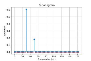
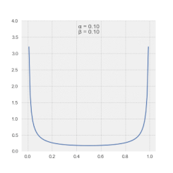
Magnitudes in the LSSA spectrum depict the contribution of a frequency or period to the variance of the time series.[4] Generally, spectral magnitudes thus defined enable the output's straightforward significance level regime.[25] Alternatively, spectral magnitudes in the Vaníček spectrum can also be expressed in dB.[26] Note that spectral magnitudes in the Vaníček spectrum follow β-distribution.[27]
Inverse transformation of Vaníček's LSSA is possible, as is most easily seen by writing the forward transform as a matrix; the matrix inverse (when the matrix is not singular) or pseudo-inverse will then be an inverse transformation; the inverse will exactly match the original data if the chosen sinusoids are mutually independent at the sample points and their number is equal to the number of data points.[17] No such inverse procedure is known for the periodogram method.
Implementation
The LSSA can be implemented in less than a page of MATLAB code.[28] In essence:[16]
"to compute the least-squares spectrum we must compute m spectral values ... which involves performing the least-squares approximation m times, each time to get [the spectral power] for a different frequency"
I.e., for each frequency in a desired set of frequencies, sine and cosine functions are evaluated at the times corresponding to the data samples, and dot products of the data vector with the sinusoid vectors are taken and appropriately normalized; following the method known as Lomb/Scargle periodogram, a time shift is calculated for each frequency to orthogonalize the sine and cosine components before the dot product;[17] finally, a power is computed from those two amplitude components. This same process implements a discrete Fourier transform when the data are uniformly spaced in time and the frequencies chosen correspond to integer numbers of cycles over the finite data record.
This method treats each sinusoidal component independently, or out of context, even though they may not be orthogonal to data points; it is Vaníček's original method. In addition, it is possible to perform a full simultaneous or in-context least-squares fit by solving a matrix equation and partitioning the total data variance between the specified sinusoid frequencies.[17] Such a matrix least-squares solution is natively available in MATLAB as the backslash operator.[29]
Furthermore, the simultaneous or in-context method, as opposed to the independent or out-of-context version (as well as the periodogram version due to Lomb), cannot fit more components (sines and cosines) than there are data samples, so that:[17]
"...serious repercussions can also arise if the selected frequencies result in some of the Fourier components (trig functions) becoming nearly linearly dependent with each other, thereby producing an ill-conditioned or near singular N. To avoid such ill conditioning it becomes necessary to either select a different set of frequencies to be estimated (e.g., equally spaced frequencies) or simply neglect the correlations in N (i.e., the off-diagonal blocks) and estimate the inverse least squares transform separately for the individual frequencies..."
Lomb's periodogram method, on the other hand, can use an arbitrarily high number of, or density of, frequency components, as in a standard periodogram; that is, the frequency domain can be over-sampled by an arbitrary factor.[3] However, as mentioned above, one should keep in mind that Lomb's simplification and diverging from the least squares criterion opened up his technique to grave sources of errors, resulting even in false spectral peaks.[19]
In Fourier analysis, such as the Fourier transform and discrete Fourier transform, the sinusoids fitted to data are all mutually orthogonal, so there is no distinction between the simple out-of-context dot-product-based projection onto basis functions versus an in-context simultaneous least-squares fit; that is, no matrix inversion is required to least-squares partition the variance between orthogonal sinusoids of different frequencies.[30] In the past, Fourier's was for many a method of choice thanks to its processing-efficient fast Fourier transform implementation when complete data records with equally spaced samples are available, and they used the Fourier family of techniques to analyze gapped records as well, which, however, required manipulating and even inventing non-existent data just so to be able to run a Fourier-based algorithm.
See also
- Non-uniform discrete Fourier transform
- Orthogonal functions
- SigSpec
- Sinusoidal model
- Spectral density
- Spectral density estimation, for competing alternatives
References
- ^ Cafer Ibanoglu (2000). Variable Stars As Essential Astrophysical Tools. Springer. ISBN 0-7923-6084-2.
- ^ a b D. Scott Birney; David Oesper; Guillermo Gonzalez (2006). Observational Astronomy. Cambridge University Press. ISBN 0-521-85370-2.
- ^ a b c d e Press (2007). Numerical Recipes (3rd ed.). Cambridge University Press. ISBN 978-0-521-88068-8.
- ^ a b c P. Vaníček (1 August 1969). "Approximate Spectral Analysis by Least-squares Fit" (PDF). Astrophysics and Space Science. 4 (4): 387–391. Bibcode:1969Ap&SS...4..387V. doi:10.1007/BF00651344. OCLC 5654872875. S2CID 124921449.
- ^ a b P. Vaníček (1 July 1971). "Further development and properties of the spectral analysis by least-squares fit" (PDF). Astrophysics and Space Science. 12 (1): 10–33. Bibcode:1971Ap&SS..12...10V. doi:10.1007/BF00656134. S2CID 109404359.
- ^ J. Taylor; S. Hamilton (20 March 1972). "Some tests of the Vaníček Method of spectral analysis". Astrophysics and Space Science. 17 (2): 357–367. Bibcode:1972Ap&SS..17..357T. doi:10.1007/BF00642907. S2CID 123569059.
- ^ a b M. Omerbashich (26 June 2006). "Gauss-Vanicek spectral analysis of the Sepkoski compendium: no new life cycles". Computing in Science & Engineering. 8 (4): 26–30. arXiv:math-ph/0608014. Bibcode:2006CSE.....8d..26O. doi:10.1109/MCSE.2006.68.
- ^ Hans P. A. Van Dongen (1999). "Searching for Biological Rhythms: Peak Detection in the Periodogram of Unequally Spaced Data". Journal of Biological Rhythms. 14 (6): 617–620. doi:10.1177/074873099129000984. PMID 10643760. S2CID 14886901.
- ^ a b c Lomb, N. R. (1976). "Least-squares frequency analysis of unequally spaced data". Astrophysics and Space Science. 39 (2): 447–462. Bibcode:1976Ap&SS..39..447L. doi:10.1007/BF00648343. S2CID 2671466.
- ^ a b c d e Scargle, J. D. (1982). "Studies in astronomical time series analysis. II - Statistical aspects of spectral analysis of unevenly spaced data". Astrophysical Journal. 263: 835. Bibcode:1982ApJ...263..835S. doi:10.1086/160554.
- ^ David Brunt (1931). The Combination of Observations (2nd ed.). Cambridge University Press.
- ^ Barning, F. J. M. (1963). "The numerical analysis of the light-curve of 12 Lacertae". Bulletin of the Astronomical Institutes of the Netherlands. 17: 22. Bibcode:1963BAN....17...22B.
- ^ a b Pascal Vincent; Yoshua Bengio (2002). "Kernel Matching Pursuit" (PDF). Machine Learning. 48: 165–187. doi:10.1023/A:1013955821559.
- ^ Y. C. Pati, R. Rezaiifar, and P. S. Krishnaprasad, "Orthogonal matching pursuit: Recursive function approximation with applications to wavelet decomposition," in Proc. 27th Asilomar Conference on Signals, Systems and Computers, A. Singh, ed., Los Alamitos, CA, USA, IEEE Computer Society Press, 1993
- ^ a b Korenberg, M. J. (1989). "A robust orthogonal algorithm for system identification and time-series analysis". Biological Cybernetics. 60 (4): 267–276. doi:10.1007/BF00204124. PMID 2706281. S2CID 11712196.
- ^ a b Wells, D.E., P. Vaníček, S. Pagiatakis, 1985. Least-squares spectral analysis revisited. Department of Surveying Engineering Technical Report 84, University of New Brunswick, Fredericton, 68 pages, Available at [1].
- ^ a b c d e f g Craymer, M.R., The Least Squares Spectrum, Its Inverse Transform and Autocorrelation Function: Theory and Some Applications in Geodesy, Ph.D. Dissertation, University of Toronto, Canada (1998).
- ^ William J. Emery; Richard E. Thomson (2001). Data Analysis Methods in Physical Oceanography. Elsevier. ISBN 0-444-50756-6.
- ^ a b Zhou, W.-X.; Sornette, D. (October 2001). "Statistical significance of periodicity and log-periodicity with heavy-tailed correlated noise". International Journal of Modern Physics C. 13 (2): 137–169. arXiv:cond-mat/0110445. Bibcode:2002IJMPC..13..137Z. doi:10.1142/S0129183102003024. S2CID 8256563.
- ^ M. Zechmeister; M. Kürster (March 2009). "The generalised Lomb–Scargle periodogram. A new formalism for the floating-mean and Keplerian periodograms". Astronomy & Astrophysics. 496 (2): 577–584. arXiv:0901.2573. Bibcode:2009A&A...496..577Z. doi:10.1051/0004-6361:200811296. S2CID 10408194.
- ^ Andrew Cumming; Geoffrey W. Marcy; R. Paul Butler (December 1999). "The Lick Planet Search: Detectability and Mass Thresholds". The Astrophysical Journal. 526 (2): 890–915. arXiv:astro-ph/9906466. Bibcode:1999ApJ...526..890C. doi:10.1086/308020. S2CID 12560512.
- ^ Korenberg, Michael J.; Brenan, Colin J. H.; Hunter, Ian W. (1997). "Raman Spectral Estimation via Fast Orthogonal Search". The Analyst. 122 (9): 879–882. Bibcode:1997Ana...122..879K. doi:10.1039/a700902j.
- ^ Palmer, David M. (2009). "A Fast Chi-squared Technique For Period Search of Irregularly Sampled Data". The Astrophysical Journal. 695 (1): 496–502. arXiv:0901.1913. Bibcode:2009ApJ...695..496P. doi:10.1088/0004-637X/695/1/496. S2CID 5991300.
- ^ "David Palmer: The Fast Chi-squared Period Search".
- ^ Beard, A.G., Williams, P.J.S., Mitchell, N.J. & Muller, H.G. A special climatology of planetary waves and tidal variability, J Atm. Solar-Ter. Phys. 63 (09), p.801–811 (2001).
- ^ Pagiatakis, S. Stochastic significance of peaks in the least-squares spectrum, J of Geodesy 73, p.67-78 (1999).
- ^ Steeves, R.R. A statistical test for significance of peaks in the least squares spectrum, Collected Papers of the Geodetic Survey, Department of Energy, Mines and Resources, Surveys and Mapping, Ottawa, Canada, p.149-166 (1981)
- ^ Richard A. Muller; Gordon J. MacDonald (2000). Ice Ages and Astronomical Causes: Data, spectral analysis and mechanisms (1st ed.). Springer Berlin Heidelberg. Bibcode:2000iaac.book.....M. ISBN 978-3-540-43779-6. OL 20645181M. Wikidata Q111312009.
- ^ Timothy A. Davis; Kermit Sigmon (2005). MATLAB Primer. CRC Press. ISBN 1-58488-523-8.
- ^ Darrell Williamson (1999). Discrete-Time Signal Processing: An Algebraic Approach. Springer. ISBN 1-85233-161-5.
External links
- LSSA package freeware download, FORTRAN, Vaníček's least-squares spectral analysis method, from the University of New Brunswick.
- LSWAVE package freeware download, MATLAB, includes the Vaníček's least-squares spectral analysis method, from the U.S. National Geodetic Survey.